Autonomous driving is undoubtedly the future of transportation. The comfort that it brings us is what drives us to work on making it real. We already have autonomous systems in public transportation in abundance, but it is different when we talk about the car roads. Driving a car requires near-human intelligence due to the nature of the environment, in fact it is impossible to define the environment. A train’s or subways’s environment can be defined mathematically and hence controlled easly, but for a machine to drive a car, it has to understand what we understand, and what we understand is even hard to define ourselves.
Computer science has come a long way, and we have already seen the rise of artificial intelligence algorithms and their effectiveness. Out of these methods Deep Learning and Convolutional Neural Networks are key tools in achieving our goal. With these algorithms computers learn general concepts of the world, and this is essential to make a safe autonomous driving (AD) system. We will see in this work briefly what they are and how they work.
Some notable companies have already achieved a high level of AD, most notably Tesla, and another AD supplier MobilEye. These companies use algorithms that are developed globally and publicly and I used them in the algorithm to partly achieve what they have achieved.
In this work I create a Scene Understanding system specialized for driving situations. I choose to evaluate the system on a virtual car driving simulation called CARLA Sim, that is going to benefit us to measure our rate of success.
I researched how existing autonomous driving systems have been built, and inspired by them I designed a system that is capable of recognizing important information for a car on the road. I used stereo imaging of multiple RGB cameras mounted on top of our virtual car for depth estimation and used trained Convolutional Neural Networks to then perform further infomration extraction from the images and perform detection for each frame of the simulation. I made a 3D webvisualizer that is able to show us the difference between ground truth information extracted programatically from the simulator and the detection infomration while simultaneously play a montage video of the simulation. Finally I evaluated the system and measured it’s validity for real situations and provided further improvement notes on my work.
I am passionate about artificial intelligence and as much inspired by the work of tech companies such as Tesla. Tesla has managed create cutting edge technology, creating compelling and practical electric cars combined with their Tesla Autopilot system. It has become iconic to sit in a Tesla and watch it drive itself. Tesla has already driven 3 billion kilometers on autopilot, their access to data is most likely number one in the world. There are other important companies who develop autopilot systems, one of them is MobilEye an Israeli subsidiary of Intel corporation that was actually a supplier of Tesla until they set apart in part due to disagreements on how the technology should be built, which is an important topic that will be discussed in the thesis.
There are a couple of topics we should establish first. The first being levels of autopilot systems as defined by SAE (Society of Automotive Engineers).
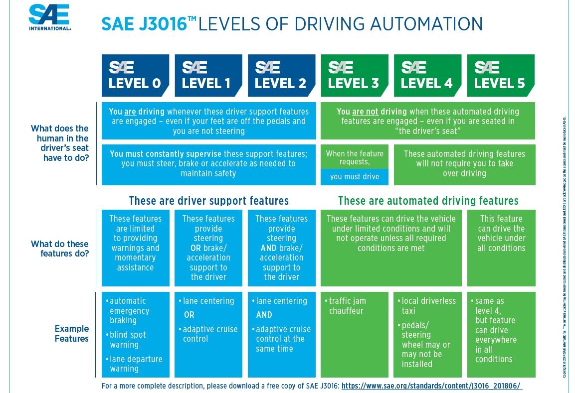
Levels of driving automation defined in SAE J3016 (“J3016B: Taxonomy and Definitions for Terms Related to Driving Automation Systems for on-Road Motor Vehicles - SAE International” 2020)
From level 0 to 2 are automations where the human is still required to fully monitor the driving environment. Tesla’s autopilot is Level 2 which is partial automation that includes control of steering and both acceleration and deceleration. From Level 3 the human is not required to monitor the environment. Full automation, where the driver is not expected to intervene and the vehicle is able to handle all situations is on Level 5. In order to achieve that level the autopilot must fully understand the environment.
This is however difficult. The algorithms that we know today are not enough to achieve understanding of the environment yet. Even Convolutional Neural Networks (CNNs) are not cabale of understanding deep concepts of the world. CNNs are mainly used in computer vision and are useful when we want to recognize patterns that appear anywhere in 2D images. Today we are able to calssify images, detect and localize objects, segment images to high accuracy, however this doesn’t mean the computer understands the scenes. Furthermore these algorithms are trained specifically: To build a detection neural network (NN) first a meticulous dataset must be created that tells the algorithm what must be detected - we call this the ground truth, or training data set. Then the NN must be trained and optimized until it yields a low error on the test dataset. We call this Deep Learning due to the fact that the networks contain millions of parameters that are trained through hundreds of thousands of iterations. This is not close to what might be general AI.
In this sense we can argue about the meaning of “scene understanding”. There is research going on in the direction of general AI most notably in my opinion by Yann LeCun the chief at Facebook AI and professsor at NYU, who works on a concept called energy-based models. The Energy-based model that is a form of generative model allows a mathematical “bounding” or “learning” of a data distribution in any dimension. Upon prediciton the model tries to generate a possible future for the current model in time, where the generated future model acts as the prediciton itself. Generative adversarial networks are a type of these models. This is in contrast to the other main machine learning approach that is the discriminative model which is what we use mostly. Perceptrons such as NNs and CNNs, support vector machines fall into this category, however the distinction is not clear.
For the purpouse of this thesis it is important to define what a system capabale of understanding scences in driving situations means. The essentials are the following:
Lane and path detection
Driveable area detection
Object detection: cars, pedestrians, etc.
Object localization in 3D real world space
Object tracking and identification
Foreign object detection: anything that shouldn’t be where it is
Traffic light and sign understanding
Handling occlusion of objects
Pedestrian crossing detection
Knowledge of surroundings and road, for example with the help of high definition maps
In an ideal world, where all cars are autonomous these perceptions would be enough, however the future of self-driving cars is going to be a transition, where both humans and machines will drive on the roads. We humans already account for each other (we try as we can), but self-driving cars will have to account for us too. We might not be smart but driving on the road sometimes requires improvization to save a situation and we might need a more general AI.
For the vehicle to understand it’s surroundigs first of all it needs sensors. Each company goes differently about the sensor suite, and it is quite interesting to examine each solution. This will be discussed in the chapter Other solutions.
In order to develop the proposed system, a sizeable dataset is needed. There are many datasets available on the internet for car driving. They include object detections, segmentations, map data, LiDAR data. Some of the most notable ones are the nuScenes dataset (Caesar et al. 2019), Waymo dataset (Sun et al. 2019) from Google’s self-driving car company or the Cityscapes dataset (Cordts et al. 2016) and more. Each of these datasets are good, however they are not really helpful for our case.
In order to localize objects in 3D space I use stereo imaging. Each AD system today employs stereo camera setting because it is a simple and cheap but accurate way of estimating depth for each pixel in an image. In order to have the freedom to create a custom camera setting I cannot rely on these datasets. Furthermore, I want to measure the success rate of my detector however there is no dataset that contains all the necessary information, because in fact it is not possible to collect everything from the real world.
This is why I choose to use a simulation instead to test the system. Using a simulation gives a huge ammount of freedom. My research work started in looking for simulators that let me extract data from the simulation in each frame and let’s me create custom world scenario and sensor settings.
After an extensive research of self-driving car simulators I found CARLA Simulator (Dosovitskiy et al. 2017) (a screenshot is seen on ) to be the most advanced one that is also opensource. CARLA is a quite mature simulator with an API that fulfills our requirements.
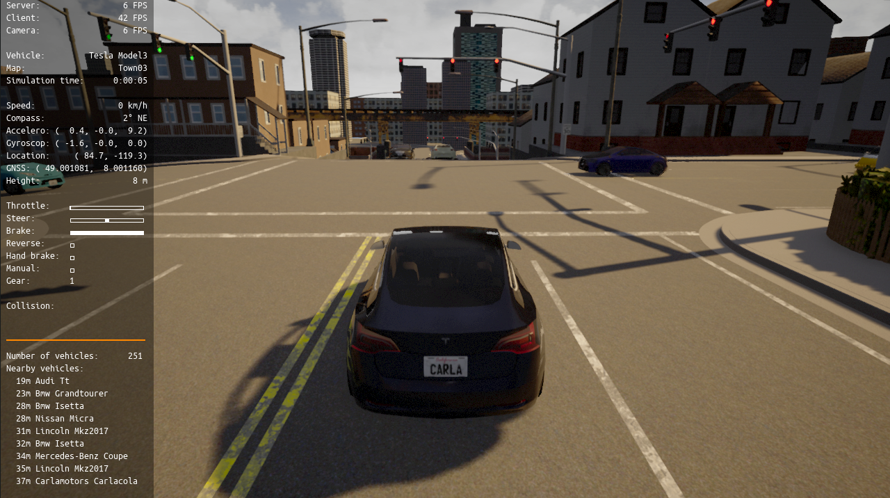
A screenshot from CARLA
I set up the virtual vehcile with 10 RGB cameras mounted on the roof creating 4 stereo sides as shown on . As the title of the thesis says, I only used RGB cameras and no other sensors. Tesla additionally uses radar and sonar sensors taking contrary to almost all other players in the field who also employ a LiDAR sensor for depth data including MobilEye and Waymo. LiDAR data is good for correction, but it is better if the AI can equally perform using only RGB cameras, since it is a more general solution that is closer to how we humans percieve the environment.
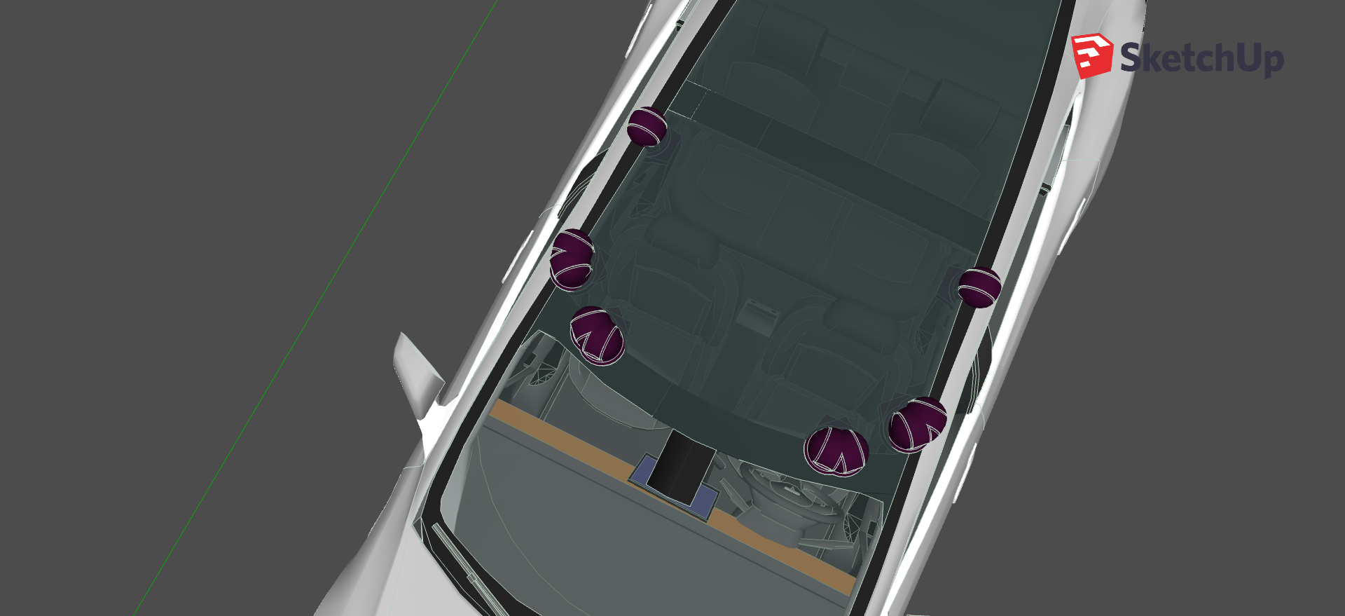
How the cameras are set up on the roof
The detector uses state-of-the-art detection, localization and segmentation model Detectron2 (Wu et al. 2019) a MASK R-CNN conv net model based on Residual neural networks and Feature Pyramid Networks trained on the COCO (Lin et al. 2014) general dataset.
Finally I develop a 3D webvisualizer that lets us replay the ground truth and detection log simultaneously and compare the error between the two. depicts this taskflow.
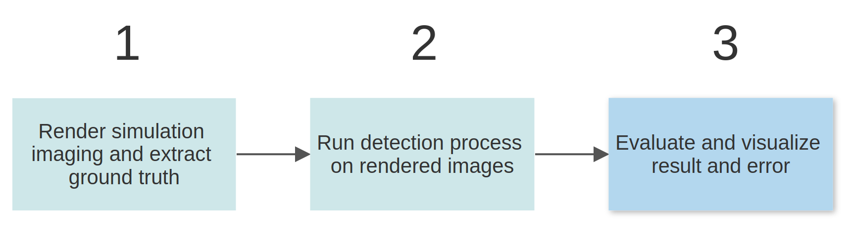
Task flow
The result is a detector that is capable of localizing vehicles, and pedestrians on the road up to 100 meters with an accuracy of ~1m in an angle of 270centered to the front. The algorithm is written in Python and uses PyTorch, with that on an NVIDIA Titan X GPU the detector can perform in 2.7FPS for one side, ie. for two cameras. In an embedded optimized system using C or C++ code this can easily be improved to even 60FPS creating a real-time system. The code cannot perform lane detection yet, but that would have been the easier part. The webvisualizer let’s us relplay the simulation frame by frame and see the detection error for each actor in the scene. It also shows a montage the original, detection and depthmap. Below, shows a screenshot of the webvisualizer in action.
3D wevisualizer
All of the code for the thesis, detector, simulator configuration and webvisualizer is available on https://github.com/najibghadri/msc-thesis and you can access the webvisualizer and interactively replay and test simulations on https://najibghadri.com/msc-thesis/.
In chapter Sensors I give an overview of the widely used sensors for peception in the automotive industry: RGB cameras, radar, LiDAR and ultrasonic sensors. In chapter Computer vision I talk about different kinds of perceptions, state-of-the-art Convolutional Networks and computer vision algorithms that are useful for our use-case.
In chapter Other solutions, I analyze Tesla’s self-driving car solution. In chapter CARLA Simulator, I introduce CARLA Simulator and some notable features of it.
In chapter Assumptions made and limitations I define the technical assumptions that I made in order to simplify the task and describe the resulting limitations.
Chapter Design and implementation details the design and implementation of the simulator configuration, the detector algorithm and the webvisualizer.
In chapter Results I present different measurements and results, then I discuss ways to improve the system in chapter Improvement notes. In chapter Experimental results I present experimentations that ended up not being part of the detection and finally close with a conclusion.
Selecting the right sensors to understand the environment is half the task. Combining multiple sensors to collect data for further information extraction is called sensor fusion. This chapter details the most widely used sensors for scene understanding for autonomous vehicles and compare them.
Radar, utrasonic and LiDAR sensors basically all work the same: emit a wave, wait until it returns and estimate the distance based on the time difference, and estimate the speed calculating the frequency shift - this is the Doppler effect: an increase in frequency corresponds to an object approaching and vice versa. A visualization is seen on .
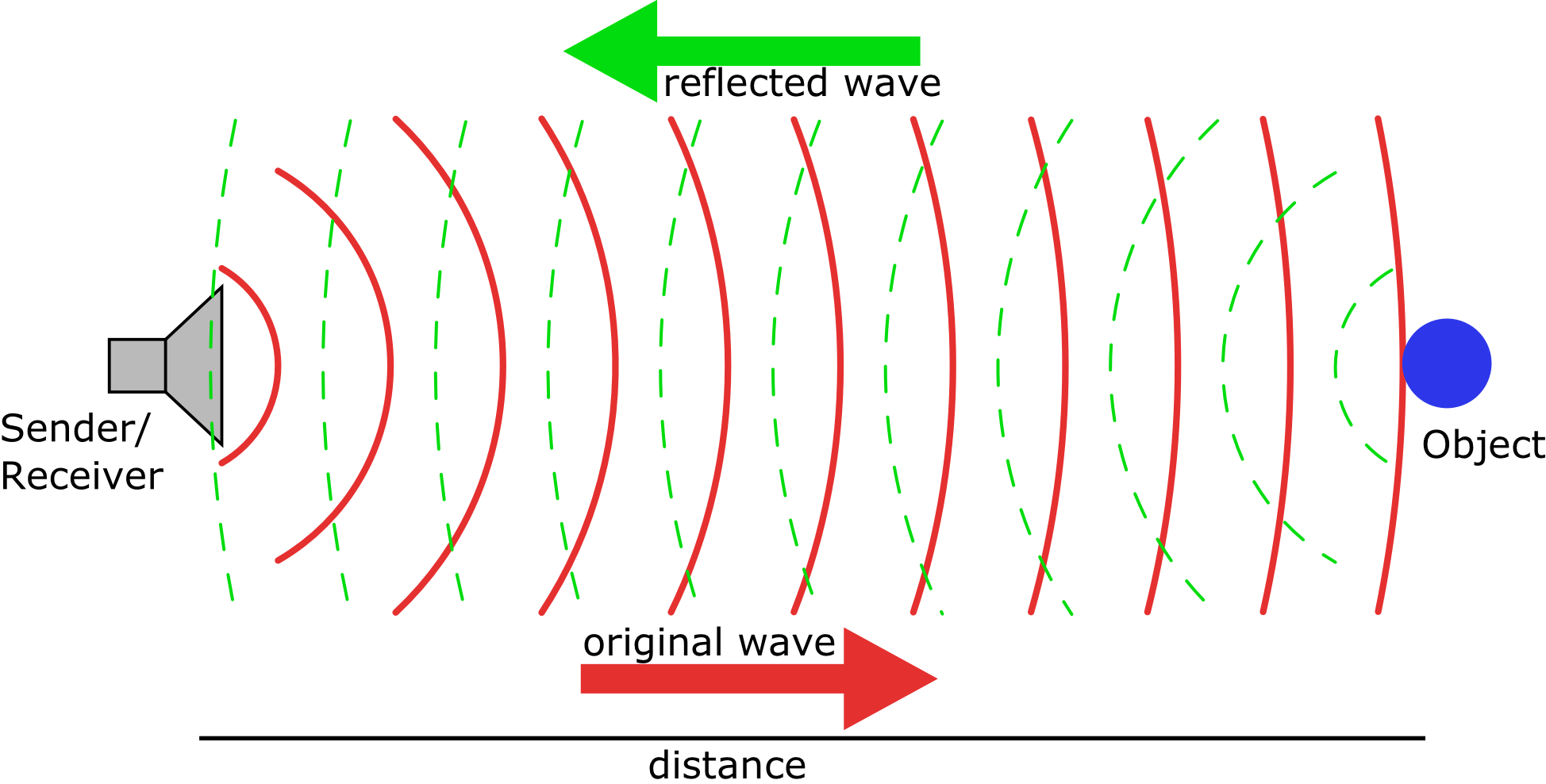
Sensing object with wave emission and reflection
Thus calculating the distance is a simple equation:
\[\begin{aligned} Distance=\frac{Speed\; of\; wavefrom * Time\; of\; Flight}{2}\end{aligned}\]
However they use different waves: Radar works with electromagnetic waves, ultrasonic sensors work with sound waves and LiDAR works with laser light.
Radar sensors at the front, rear and sides have become an essential component in modern production vehicles. Though most frequently used as part of features like parking assistance and blind-spot detection, they have the capability to detect objects at much greater range – several hundred meters in fact.
Radar sensors are excellent at detecting objects, but they’re also excellent for backing up other sensors. For instance, a front-facing camera can’t see through heavy weather. On the other hand, radar sensors can easily penetrate fog and snow, and can alert a driver about conditions obscured by poor conditions. Radar is robust in harsh environments (bad light, bad weather, extreme temperatures).
Automotive radar sensors can be divided into two categories: short-range radar (SRR), and long-range radar (LRR). The combination of these types of radar provides valuable data for advanced driver assistance systems.
Short-range radar (SRR) Short-range radar (SRR): Short-range radars (SRR) use the 24 GHz frequency and are used for short range applications like blind-spot detection, parking aid or obstacle detection and collision avoidance. These radars need a steerable antenna with a large scanning angle, creating a wide field of view.
Long-range radar (LRR) Long-range radar (LRR): Long-range radars (LRR) using the 77 GHz band (from 76-81GHz) provide better accuracy and better resolution in a smaller package. They are used for measuring the distance to, speed of other vehicles and detecting objects within a wider field of view. Long range applications need directive antennas that provide a higher resolution within a more limited scanning range. Long-range radar (LRR) systems provide ranges of 80 m to 200 m or greater.
Ultrasonic (or sonar) sensors, alike radar, can detect objects in the space around the car. Ultrasonic sensors are much more inexpensive than radar sensors, but have a limited effective range of detection. Because they’re effective at short range, sonar sensors are frequently used for parking assistance features and anti-collision safety systems. Ultrasonic sensors are also used in robotic obstacle detection systems, as well as manufacturing technology. Ultrasonic sensors are not as susceptible to interference of smoke, gas, and other airborne particles (though the physical components are still affected by variables such as heat), and they are independent of light conditions. They also work based on the reflection of emission principle.
Ultrasound signals refer to those above the human hearing range, roughly from 30 to 480 kHz. For ultrasonic sensing, the most widely used range is 40 to 70 kHz. At 58 kHz, a commonly used frequency, the measurement resolution is one centimeter, and range is up to 11 meters. At 300 kHz, the resolution can be as low as one millimeter; however, range suffers at this frequency with a maximum of about 30 cm.
As Radar is to radio waves, and sonar is to sound, LiDAR (Light Detection and Ranging) uses lasers to determine distance to objects. LiDAR sometimes is called 3D laser scanning. It does this by spinning a laser across its field of view and measuring the individual distances to each point that the laser detects. This creates an extremely accurate (within 2 centimeters) 3D scan of the world around the car.
The principle behind LiDAR is really quite simple. Shine a small light at a surface and measure the time difference it takes to return to its source. The equipment required to measure this needs to operate extremely fast. The LiDAR instrument fires rapid pulses of laser light at a surface, some at up to 150,000 pulses per second. A sensor on the instrument measures the amount of time it takes for each pulse to bounce back. Light moves at a constant and known speed so the LiDAR instrument can calculate the distance between itself and the target with high accuracy. By repeating this in quick succession the insturment builds up a complex ’map’ of the surface it is measuring.
The three most common currently used or explored wavelengths for automotive LiDAR are 905 nm, 940 nm and 1550 nm, each with its own advantages and drawbacks.
LiDAR sensors are able to paint a detailed 3D point cloud of their environment from the signals that bounce back instantaneously. It provides shape and depth to surrounding cars and pedestrians as well as the road geography. And, like radar, it works just as well in low-light conditions.
You can see how a LiDAR sensor from Luminar1 reconstructs the environment in .
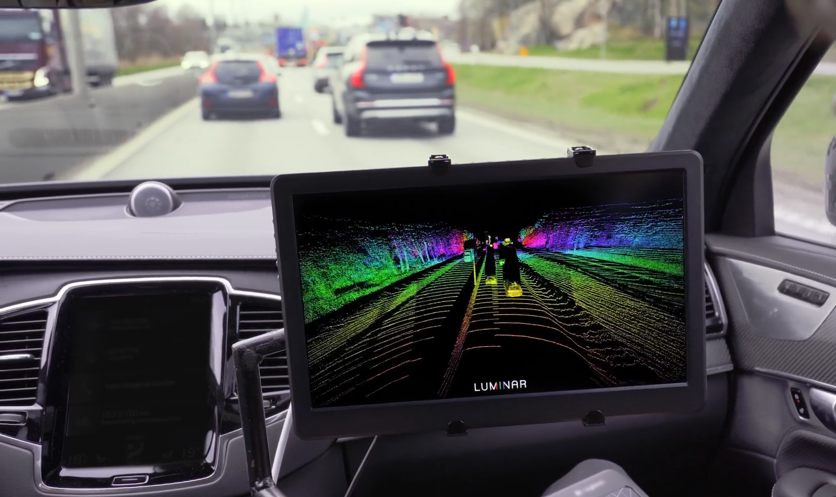
Luminar LiDAR in action
Currently, LiDAR units are big, and fairly expensive - as much as 10 times the cost of camera and radar — and have a more limited range. You will most often see them mounted on Mapping Vehicles, but as the technology becomes cheaper, we might see them on trucks and high-end cars in the near future.
Cameras are the essential sensors for self-driving cars. Most imaging sensors are sensitive from about 350 nm to 1000 nm wavelengths. The most common types of sensors for cameras are CCD (charged coupled device) and CMOS (complementary metal–oxide–semiconductor). The main difference between CCD and CMOS is how they transfer the charge out of the pixel and into the camera’s electronics.
CCD-based image sensors currently offer the best available image quality, and are capable of high resolutionsm making them the prevalent technology for still cameras and camcorders.
An important aspect of cameras is the camera model that describes how points of the world translate to pixels in the image. That is going to be essential when we want to apply the inverse projection to determine the world-position of objects in the picture. This will be discussed in the following chapters.
Originally introduced for military applications in 1974, GPS probes today can be found in cameras, watches, key fobs, and of course, the smartphone in our pockets.
The lesser-known WPS stands for Wi-Fi Positioning System, which operates similarly. When a probe detects satellites (GPS) or Wi-Fi networks (WPS), it can determine the distance between itself and each of those items to render a latitude and longitude. The more devices a GPS/WPS probe can detect, the more accurate the results. On average, GPS is only accurate to around 20 meters.
For WPS the most common and widespread localization technique is based on measuring the intensity of the received signal, and the method of “fingerprinting”. Typical parameters useful to geolocate the wireless access point include its SSID and MAC address. The accuracy depends on the number of nearby access points whose positions have been entered into the database. The Wi-Fi hotspot database gets filled by correlating mobile device GPS location data with Wi-Fi hotspot MAC addresses.
After collecting data from the sensors we choose we need to implement the right algorithms to extract information from the sensor data. In this chapter I start with explaining the basics of computer vision and then move on to advanced convolutional neural netowrks that will help our goal.
Computer Vision, often abbreviated as CV, is defined as a field of study that seeks to develop techniques to help computers “see” and understand the content of digital images such as photographs and videos.
The problem of computer vision appears simple because it is trivially solved by people, even babies. Nevertheless, it largely remains an unsolved problem based both on the limited understanding of biological vision and because of the complexity of vision perception in a dynamic and nearly infinitely varying physical world.
Image classification is considered to be the most basic application of computer vision. The rest of the developments in computer vision are achieved by making small enhancements on top of this. Since this task is intuitive for us, we fail to appreciate the key challenges involved when we try to design systems similar to our eye. Some challenges for computers are:
Variations in viewpoint
Difference in illumination
Hidden parts of images, occulsion
Background Clutter
Various techniques, other than deep learning are available in computer vision. They work well for simpler problems, but as the data becomes huge and the task becomes more complex, they are no substitute for deep CNNs. Let’s briefly discuss two simple approaches.
In the KNN algorithm each image is matched with all images in training data. The top K with minimum distances are selected. The majority class of those top K is predicted as output class of the image. Various distance metrics can be used like L1 distance (sum of absolute distance), L2 distance (sum of squares), etc. However KNN performs poorly - qute expectedly - they have a high error rate on complex images, because all they do is compare pixel values among other images, without any use of image patterns.
They use a parametric approach where each pixel value is considered as a parameter. It’s like a weighted sum of the pixel values with the dimension of the weights matrix depending on the number of outcomes. Intuitively, we can understand this in terms of a template. The weighted sum of pixels forms a template image which is matched with every image. This will also face difficulty in overcoming the challenges discussed in earlier as it is difficult to design a single template for all the different cases.
Visual recognition tasks such as image classification, localization, and detection are key components of computer vision. However these are not possible to achieve with traditional vision.
Recent developments in neural networks and deep learning approaches have greatly advanced the performance of these state-of-the-art visual recognition systems.
Neural networks are the basis of deep learning methods. They are made up of multiple layers, each layer containing multiple perceptrons. Layers can be fully-connected or sparsely if possible, providing some performance benefits. Each perceptron is an activation function whose input is the weighted output of perceptrons from previous layers, and the function is usually a sigmoid function. A neural network’s first layer is the input layer and the last layer is the output, which could be an array of perceptron where only one yields a high output creating a classifier. Layer in-between are called hidden layers and it is up to design and experimentation the determine what is the right configuration of hidden layers.
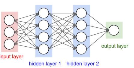
Neural network visualization. Image taken from CS231N Notes
Neural Networks (NN) are good at classifying different patterns recieved in the input layers however they are not sufficient for even image classification, because in one part the number of inputs is way to high. Consider a high resolution image with \(1000\times 1000\times 3\) pixels, then the NN has 3million input parameters to process. This takes a long time and too much computational power.
Secondly the neural network architecture in itself is not a general-enough solution (if you think about it, it is similar to a linear classifier or a KNN).
Convolutional Neural Network (CNNs) however solve image classification and more. A CNN is able to capture the spatial features in an image through the application of relevant filters. The architecture performs a better fitting to an image dataset due to the reduction in the number of parameters involved and reusability of weights.
There is material on the internet in abundance about how convolutional neural networks work, and I have read many of them, but the one I recommend most is the Stanford course CS231N2.
The general architecture of CNN is similar to a cone, where the first layer is the widest and each layer first convolves multiple filters (which in the beginning of the CNN correspond to edges and corners) applying ReLU (rectifier, non-linearity function) then it downsizes the input which is called the max pooling. This repeated over and over in the end results in a small tensor which can then be fed to the fully-connected (FC) layers (i.e. a neural network) which acts as the classifier.
Why is this the winner architecture? Because if you think about it the neural network in the end only has to vote for the presence of the right features in roughly the right image position, not for each pixel. A visualization of a CNN’s architecture can be seen in .
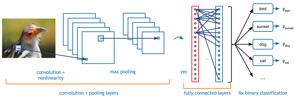
Architecture of a CNN
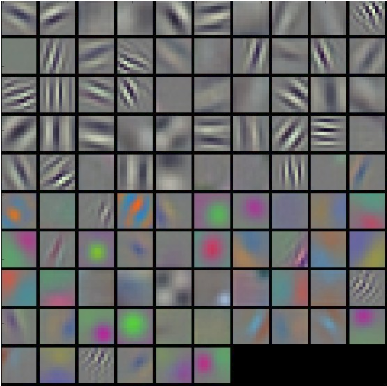
A visualization of the features learned in the first convnet layer in AlexNet (Krizhevsky, Sutskever, and Hinton 2012). AlexNet was a CNN which revolutionized the field of Deep Learning, and is built from conv layers, max-pooling layers and FC layers. Image taken from CS231N notes.
There are various architectures that have emerged each incrementally improving on the previous ones: LeNet (Lecun et al. 1998) - the work of Yann LeCun himself, AlexNet (Krizhevsky, Sutskever, and Hinton 2012) VGGNet (Simonyan and Zisserman 2014) GoogLeNet (Szegedy et al. 2014) ResNet (He et al. 2015)
Deep learning referes to the procedure of training neural networks and convolutional neural networks to perform the task at hand accurately. During deep learning first a dataset is created with training images coupled with “ground truth” data that is the required prediction for each image. The neural networks are then fed with the images in batches for a certain number of iterations - epochs. The weights of the neural network and the filters are adjusted with the loss function that comes from calculating the error of the current prediction and the ground truth for each image. This error is then “backpropagated” which is just another way of saying it is multiplied with the derivative of each weight in the network and subtracted from it. For filters this means “filtering filters”, so only those filters will stay in the convnet which resulted in a non-zero gradient in the neural network.
The task to define objects within images usually involves outputting bounding boxes and labels for individual objects. This differs from the classification / localization task by applying classification and localization to many objects instead of just a single dominant object.
If we use the Sliding Window technique like the way we classify and localize images, we need to apply a CNN to many different crops of the image.
In order to cope with this, researchers have proposed to use regions instead, which are suggestions of regions that are likely to contain objects. The first such convnet is called R-CNN (Girshick et al. 2013) (Region-based Convolutional Neural Network).
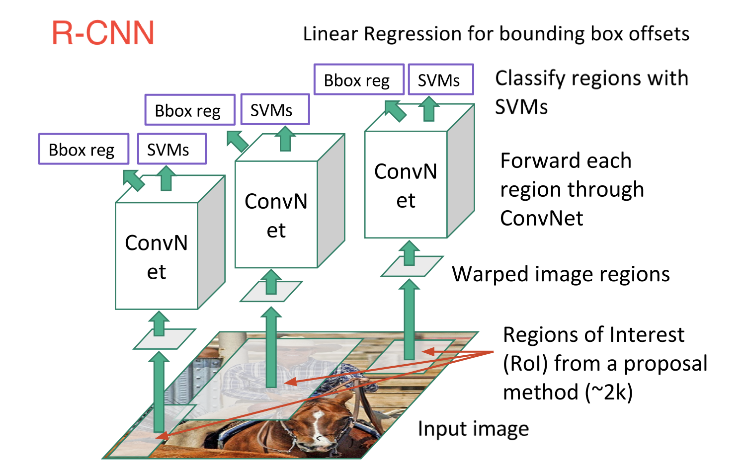
R-CNN architecture
An immediate descendant to R-CNN is Fast R-CNN (Girshick 2015), which improves the detection speed through 2 augmentations: 1) Performing feature extraction before proposing regions, thus only running one CNN over the entire image, and 2) Replacing SVM with a softmax layer, thus extending the neural network for predictions instead of creating a new model.
There are other methods for object detection and localization but in general they are all based on first feature extraction then classification with different intermediate procedures.
You Only Look Once (YOLOv4 (Bochkovskiy, Wang, and Liao 2020) being the latest)
Single Shot MultiBox Detector (SSD) (Liu et al. 2015)
Central to Computer Vision is the process of segmentation, which divides whole images into pixel groupings which can then be labelled and classified. Particularly, Semantic Segmentation tries to semantically understand the role of each pixel in the image (e.g. is it a car, a motorbike, or some other type of class?). Therefore, unlike classification, we need dense pixel-wise predictions from the models.
One of the earlier approaches was patch classification through a sliding window, where each pixel was separately classified into classes using a patch of images around it. This, however, is very inefficient computationally because we don’t reuse the shared features between overlapping patches. The solution, instead, is Fully Convolutional Networks (FCN) (Long, Shelhamer, and Darrell 2014).
Beyond Semantic Segmentation, Instance Segmentation segments different instances of classes, such as labelling 4 cars with 4 different colors. Instance segmentation problem is explored at Facebook AI using an architecture known as Mask R-CNN (He et al. 2017).
The idea is that since Faster R-CNN works so well for object detection is it possible to extend it to that is also performs pixel-level segmentation.
Mask R-CNN adss a branch to Faster R-CNN that outputs a binary mask that says whether or not a given pixel is part of an object. The branch is a Fully Convolutional Network on top of a CNN-based feature map. Detectron2 (Wu et al. 2019) a detection framework developed by Facebook, is based on Mask R-CNN and it is the framework I ended up using.
Object Tracking refers to the process of following a specific object of interest, or multiple objects, in a given scene. It traditionally has applications in video and real-world interactions where observations are made following an initial object detection. Now, it’s crucial to autonomous driving systems.
Simple Online and Realtime Tracking - SORT (Wojke, Bewley, and Paulus 2017) and Deep SORT (Wojke and Bewley 2018) Are both based on Kalman filters to use the available detections and previous predictions to arrive at a best guess of the current state. Deep SORT extends SORT with the use feature extraction with encoders. These features are then kept in a dictionary for each object. For each detection throughout the tracking process a distance is calculated between signatures in the dictionary and the current object’s feature model this way tracking previously identified objects.
It is important for a self-driving company to openly detail their technical solution because it let’s people trust their autopilot solution. However it wasn’t easy to find open information about the details of different companies, because the technology itself is in early stages. The details I found did provide inspiration on how to combine different algorithms.
The only open information I found about Tesla’s autopilot technology is their own keynote about autopilot.3
The sensor suite for tesla vehicles is seen on . Tesla uses 360RGB camera vision and sonar sensing with a radar facing forward. The sonar sensors provide depth information for the surrounding objects and the radar provides depth data for further distances.
The algorithms they use was not clear from the keynote, however I found two clips on the internet that claim to be the output of Tesla’s detection system. Based on that and the keynote it is safe to assume that they integrate the following tasks.
Object detection and 3D bounding box detection
Lane detection and path estimation
Tracking
Possibly some kind of segmentation
Traffic sign detection and understanding
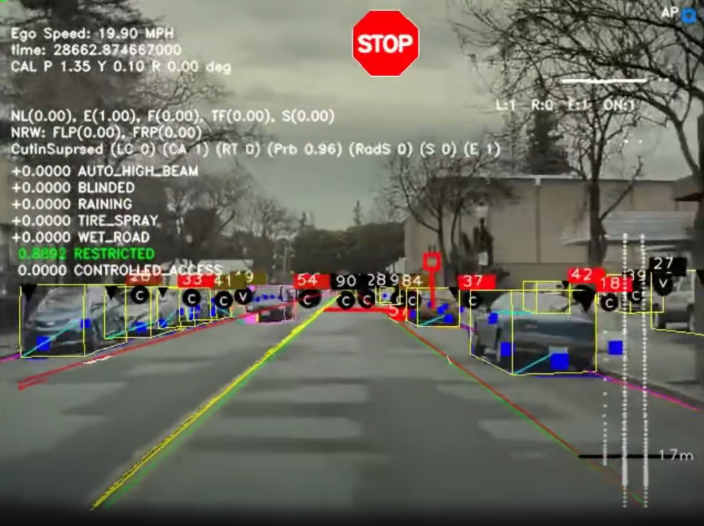
A screenshot form a clip that shows Tesla Autopilot’s perception output https://www.youtube.com/watch?v=fKXztwtXaGo
Another screenshot form a clip that shows Tesla Autopilot’s perception output https://www.youtube.com/watch?v=_1MHGUC_BzQ&t=225s
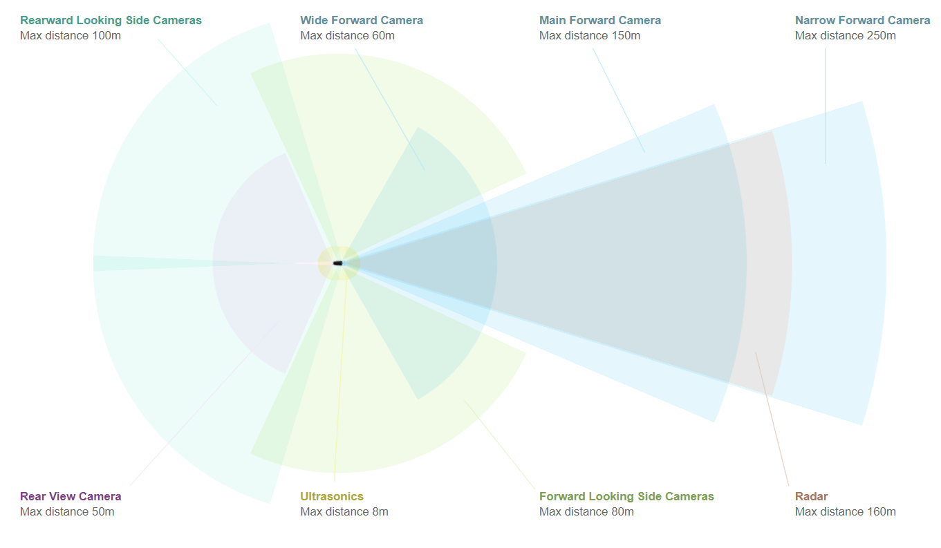
Tesla sensor suite infographic from https://www.tesla.com/autopilot
With sensor fusion they achieve depth estimation and detection thus they are able to reconstruct the scenes around the vehicle.
CARLA’s mission is to create a simulator that can simulate sufficient-enough real-world traffic scenarios so that it is more accessible for researchers like myself to research, develop and test computer vision algorithms for self-driving car.
CARLA (Dosovitskiy et al. 2017) is an open-source simulator for autonomous driving research. It is written in C++ and provides an accessible Python API to control the simulaton execution. It has been developed from the ground up to support development, training, and validation of autonomous driving systems. In addition to open-source code and protocols, CARLA provides open digital assets (urban layouts, buildings, vehicles) that were created for this purpose and can be used freely. The simulation platform supports flexible specification of sensor suites, environmental conditions, full control of all static and dynamic actors, maps generation and much more. It is developed by the Barcelonian university UAB’s computer vision CVC Lab and supported by companies such as Intel, Toyota, GM and others. The repository for the project is at https://github.com/carla-simulator
It provides scalability via a server multi-client architecture: multiple clients in the same or in different nodes can control different actors. Carla exposes a powerful API that allows users to control all aspects related to the simulation, including traffic generation, pedestrian behaviors, weathers, sensors, and much more. Users can configure diverse sensor suites including LiDARs, multiple cameras, depth sensors and GPS among others. Users can easily create their own maps following the OpenDrive standard via tools like RoadRunner. Furthermore it provides integration with ROS4 via their ROS-bridge
I used CARLA 9.8.0 in the project that was the latest at the time (2020 March 09). Carla has a primary support for Linux so I could run it easly on Ubuntu. It requires a decent GPU otherwise the simulation is going to be slow.
It’s important to mind the coordinate system used in Carla, because later when we will extract data the axes must be mapped to the correct data points. Since Carla is built with Unreal Engine5 it uses the coordinate system as in : X coordinate is to the front of the ego actor, Y is to the right of ego and Z is to the top.
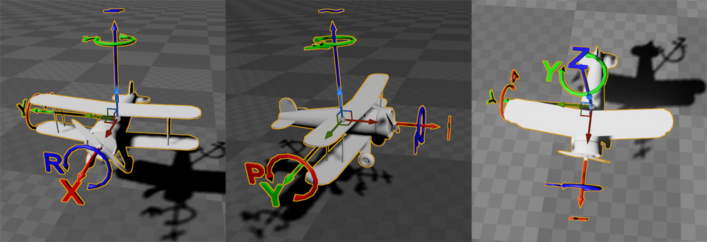
Carla coordinate system
I believe the future of self-driving car research and development is in part with simulations and in part with real-world training as well. To develop a self-driving AI from ground up it is certainly advisable to first develop and test the algorithms in a simulation.
In order to create simulations that are rich and different Carla provides a large variety of actors and maps. The traffic manager can also be parametrized to control how pedestrians and vehicles move: their speed, minimum distance, and even “aggressivity” towards each other, which means how willing are they to collide instead of waiting until the actor in front moves away. This is actually useful as it helps unlock possible traffic deadlocks. The latest CARLA provides 8 maps but in newer versions they will be adding new maps. You can see a screenshot of each rendering in the 6 maps I used in .
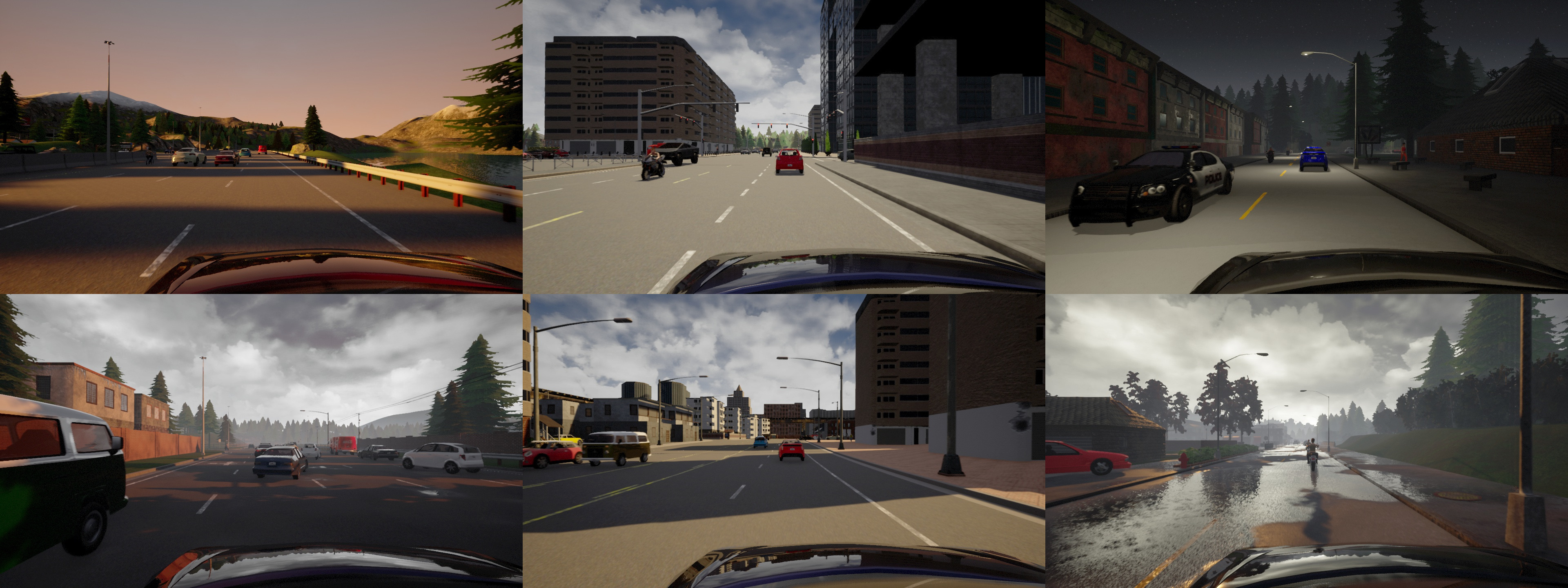
Variety of maps in Carla
A simulation obviously can’t return the variety and exact nature of scenarios that happen in nature. However I believe they are sufficient for testing an entry-level self-driving system and that with the use of simulations a company can lower the costs of development. The rise of simulators itself shows there is a need for the market.
The Carla simulator’s API support a wide range of sensors: RGB Cameras, LiDAR, Radar, GPS, gyroscope, accelerometer, compass and more. These are easy to use, If you are interested I recommend reading the sensors reference in their documentation6
Carla also provides miscellaneous sensors that help collecting ground-truth data for deep learning applications. This includes semantic segmentation camera, depthmap camera and other simple ones such as collision detector as seen in .
Different sensors and cameras in Carla (semantic segmentation, LiDAR, depthmap)
There are a couple of other dedicated projects for simulators. There is Deepdrive from Voyage auto7, an American AD supplier, NVIDIA has a project going on called Drive Constellation8 which is said to be advanced but is not opensource. Nvidia provides Harware In the Loop simulation for Drive Constellation which is an even more advanced simulation infrastructure that allows for testing the systems real-timeness. There is another project called RFPro9. However these are either not opensource or not mature enough. CARLA Simulator (Dosovitskiy et al. 2017) was by far the best one for my case.
In order to simply the task of scene understanding we need to define boundaries to measure the success of the detector.
The first essential assumption is that there will only be ideal situations which means that we will only need to detect actors that we expect on the road: vehicles, bicycles, pedestrians. In the real world foreign objects on the road are a usual and dangerous phenomenon, however here I won’t take that into account.
First of all we are going to specialize to day-light situations only. This detection with RGB cameras at night is difficult, in order to achieve that we need other sensors such as Radar, Sonar or LiDAR. As we are only using RGB cameras we arge going to assume that all driving situations occur in daylight.
Another important assumption is that the driving field and landscape area is flat. It isn’t difficult to detect object that are a bit higher on the picture but it is difficult to recognize the curvature of the plane on the image. In case the detector can interpret curvature and the ego car is on an angled road the angle data from the gyroscope sensors has to be take into account and subtracted from the percieved angles. It is generally true that inorder to recognize true information about the world the relative position and orientation has to be taken into account.
In order to reduce this complexity, we are going to only take into account the objects’ position on the x,y surface coordinates and disregard the Z coordinate on evaluating the detection. This will be discussed further in about improvements.
As described before there are many ways of detecting lane and the easiest is to use the Hough transform and detect the lanes directly in front of the car. However this is not a robust solution: this only gives good results in good illumination and weather situations. It is true that most situations are like this but there are still many unpainted roads, dirt roads or simply due to lightning and weather the lane edges won’t be clear.
One robust solution would be to take into account the vehicles in front and behind us and interpret their path as the right path and regress the lane to their path.
Another solution is to take into account previously driven paths. This is the approach Tesla takes however it is not clear how exactly.
It is important to determine the orientation of the detected cars on the road, so that the algorithm knows the depth data corresponds to which side of the detected vehicle. It is also a clue that helps in determining the direction of the car. Detecting keypoints could be done with an algorithm similar to Latent 3D Keypoints (Suwajanakorn et al. 2018) that I experimented with (see ).
Because the algorithm doesn’t take into account orientation the most straightforward way to localize an object upon detection is to take the center of it’s bounding box. We will see in the results chapter how big the resulting error is.
The final algorithm does not include tracking, this means that the identity of each detected actor/object is inconsistent throughout time. Tracking helps handling occlusion of previously detected pedestrians/vehicles and also in building up a knowledge base for each actor throughout it’s presence in the scene. This can help in estimating the actor’s velocity, acceleration and it provides a base for interpreting intentions. I simplified the task by not considering identity throughout time an important factor, eventhough in a real system it is a must-have.
The final product will be a detector that can detect vehicles and pedestrians up more than a 100 meters and localize them using stereo vison. The detector work with a reasonable accuracy error and is built in an extensible way so that tracking, and improved instance segmentator and lane detection can be plugged in. The webvisualizer then can be easily extended to show futher information by a newer version of the detector.
Let’s recap the task flow of the task I described in the Introduction: After configuring the simulator with the designed camera setting I render multiple traffic scenarios in different maps provided by CARLA while extracting all necessary information into a log file to later compare the detection log with
Task flow
Soon it became obvious that Linux operating system is the right tool to use for development. I have been using Ubuntu before this project as well so I was already familiar with everything. The main IDE I used throughout the project is Visual Studio Code, which thanks to it’s openness and community has many useful extensions that helped me develop in fact every part of the thesis: Python, Nodejs and Javascript for the webvisualizer and finally LaTeX and ofcourse git support.
I also used Conda which is I think an essential tool when you want to develop ML and AI projects with Python. Conda makes it easy to create and use separate Python environments. This is important because different implementations of algorithms require different versions of the same packages thus it keeps a clean separation. The drawback is that consecuently it requires an excessive ammount of hard-drive space.
Upon developing the algorithm and experimenting with it I used Jupyter Notebook which is a Python runtime on top of the bare one and a web-based IDE at the same time. With Jupyter Notebook it is easy to change and re run the code thanks to it’s “kernel” system, which keeps the value of variable and imported packages between executions.
For the GPU-intensive tasks such as simulation and convnet calculations in the detector I was provided with a remote Titan X GPU10 by my university.
Mounting cameras around the vehicle to have an all around vision is an essential design strategy, as we have seen in the work of other companies in . However we will need to determine depth as well. I decided to use only cameras in a stereoscopic structure to create 5 stereo sides around the vehicle. The following image shows the design setting with field of views visualized in .
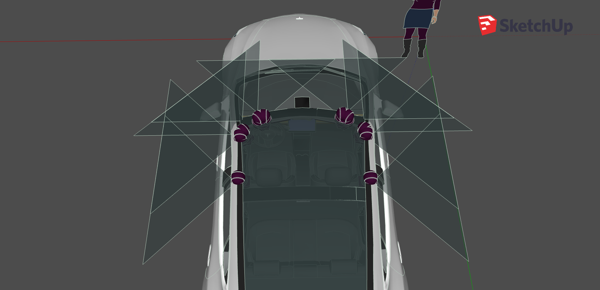
The stereo camera setting I used on top of the virtual Tesla Model 3
In details:
Front stereo: two cameras looking straight to the front 0.8 meters apart
Right corner and left corner stereo cameras: the cameras are on the diagonal corners of a 20 cm wide 20cm tall triangle creating two 45 angled stero vision.
Right and left side stereos are turned 90to the sides and they are apart 0.5 meter.
The cameras are 1.5 meters above the ground and they are mounted relative to the bottom center-point of the vehicle.
The advantage of puting stereo cameras apart to a relatively large distance is that it increases the accuracy of the stereo block matching algorithm to a further distances. The drawback however is that a smaller portion of the right and left side images are going to intersect hence creating a smaller field of view. However due to the corner stereo cameras this is not a problem for us.
Carla simulator can be ran in two time-step settings: variable and synchronous. In real-world perception it is a complex task by itself to synchronize multiple cameras with each other so that when the algorithm calculates information based on data from multiple sensors they all correspond to the same moment in time with an error boundary. In a simulation however we can have the freedom to synchronize the simulation timesteps themselves and collect all imaging data between each timestep. Setting Carla to synchronous timestep ensures that all images in a certain frame are collected and respond to the same moment.
I used 30FPS timestep setting so that physics calculations are still realistic but the performance is not too bad. We also have to account for the size of the generated images: it was good to half the size of the image datasets from a 60FPS setting. Increasing the traffic participants also degrades the performance. I usually used 200 vehicles and 100 pedestrians for each map, that resulted in realistic traffic scenarios.
I recorded different scenarios of approximately 1 minute, which means 1800 frames on 30FPS. On the Titan X machine it it took 15 minutes to render 1 simulation minute, i.e. it ran the simulation with 2FPS. Note, this is different from the simulation time-step which we fixed to 30FPS. Since I collect 10 images in each frame it results in a dataset of 18000 images.
The camera setting I used is an undistorted camera that takes \(1280\times720\) resolution images, i.e. HD 720p images, compressed with JPEG to yield a reasonable size. This way one image is on average 215 kilobytes instead of 1MB which is a good compression rate and this was the limit where I did not see any difference in detection accuracy.
In a real-world systems images go straight to the GPU and CPU unit and they get downscaled to the choosen size before feeding into the algorithm. I had to resort to compression because of the research nature of the project: I reran and tested the accuracy of the detector many times on the same dataset.
Using an undistorted camera matrix only means that we need to use one less back transformation matrix in the detection calculations. In real-world the intrinsic camera matrix is calculated and corrected for cameras that are mounted on cars and it is part of the calculation.
Besides imaging we have the ground truth log data. During the simulation, besides rendering images I coded a logger that logs the necessary information of the state of the simulator for each frame. This information is built up in a json-like dictionary, and at the end of the simulation it is saved to one file, that I call the framelist.
Naming the images in an organized way is important to make it easy to read the images in a structured way upon detection. Each image starts with the number of the frame it was taken in. Starting the simulator server Carla increases a frame counter starting with 1. To know which image corresponds to which camera, the framenumbers are postfixed with a label. shows the postfixes for each image.
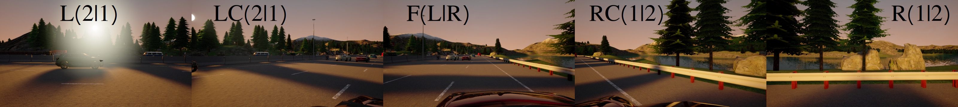
L2/1, R1/2: Right side/Left side first and second cameras, LC(2/1), RC(1/2): Right corner, left corner cameras, FL FR: Front left, front right cameras
In each frame I log information about the current state of the simulation. For the purpouses of the final detector the following information gets logged in each frame:
Frame’s number: the value of the frame counter at each frame
For all walker and vehicle actors in a 100 meter radius from the ego car:
Id: corresponds to the actor’s unique id among other actors.
Relative position: X, Y, Z coordinate of the actor in the CARLA coordinate system (see )
Distance: Euclidean distance from the ego car
Waypoints: these are center and left-right points of the lane the egocar is currently in up to 30 points forward. These were meant to be the ground-truth data for lane-detection
This information is then exported into a JSON file with the following format:
frameList: [
            {
                frame: Number,
                actors: [
                    {
                        type: car|pedestrian,
                        id: Number,
                        relative_position: {
                            x: Number,
                            y: Number,
                            z: Number,
                        }
                    },
                ],
            },
        ]
For a one-minute simulation the ground-truth json file is approximately 20 megabytes. It isn’t optimal to save information like this for longer simulations. In those cases it is recommended to use a binary format. Carla provides a way to save binary information of the recording but unfortunately there were issues with recording that way, so I ended up with this custom log format. However it ended up being beneficial, because the webvisualizer simply loads the json files (detection and ground truth) into two JavaScript objects.
The algorithm plan is the following: for each stereo pair of images calculate the disparity map with a stereo block matching algorithm. Then detetect objects and their segmentation mask (instance segmentation) with a state-of-the-art convnet and then extract the disparity data using the segmentaiton mask. Then use the extracted disparity data to estimate the depth of the detected object and then reproject to Carla-world coordinates to match the logfile coordinate system.
Detectron2’s (Wu et al. 2019) Mask R-CNN model provides both object detection and instance segmentation so I decided to use it. Detectron is built with PyTorch, Facebook’s own GPU-aided ML library.
The algorithm runs the detecton prediction only on the left image of each side, because later on we will need the segmentation mask of the left image to extract the depth data from the disparity map generated by the stereo block matching algorithm.
Before prediction if our ego car falls into the image it is filled with zeros, i.e. it is occluded ith black color. It is better to use black since it is all zeros, and therefore convnet is not going to be sensitive for those parts of the image.
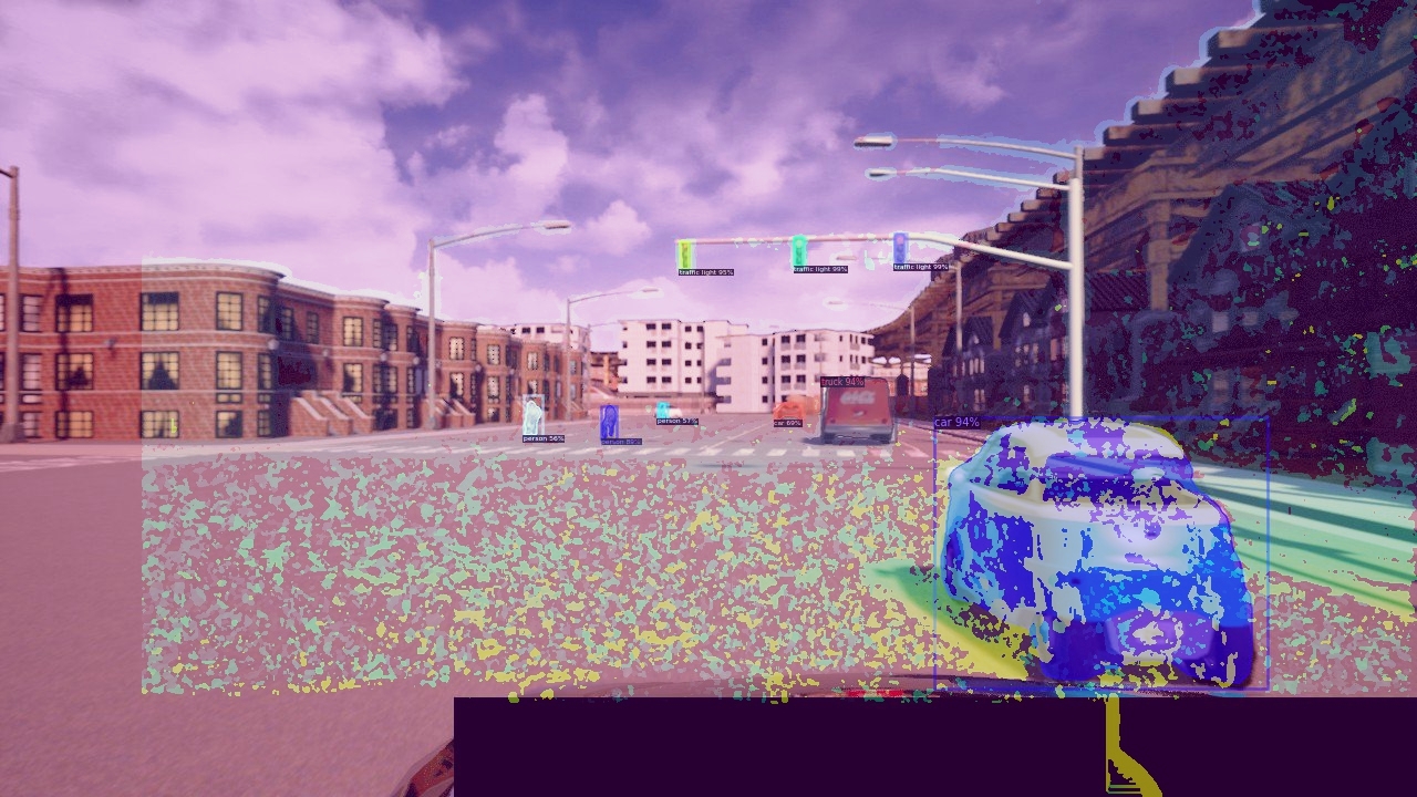
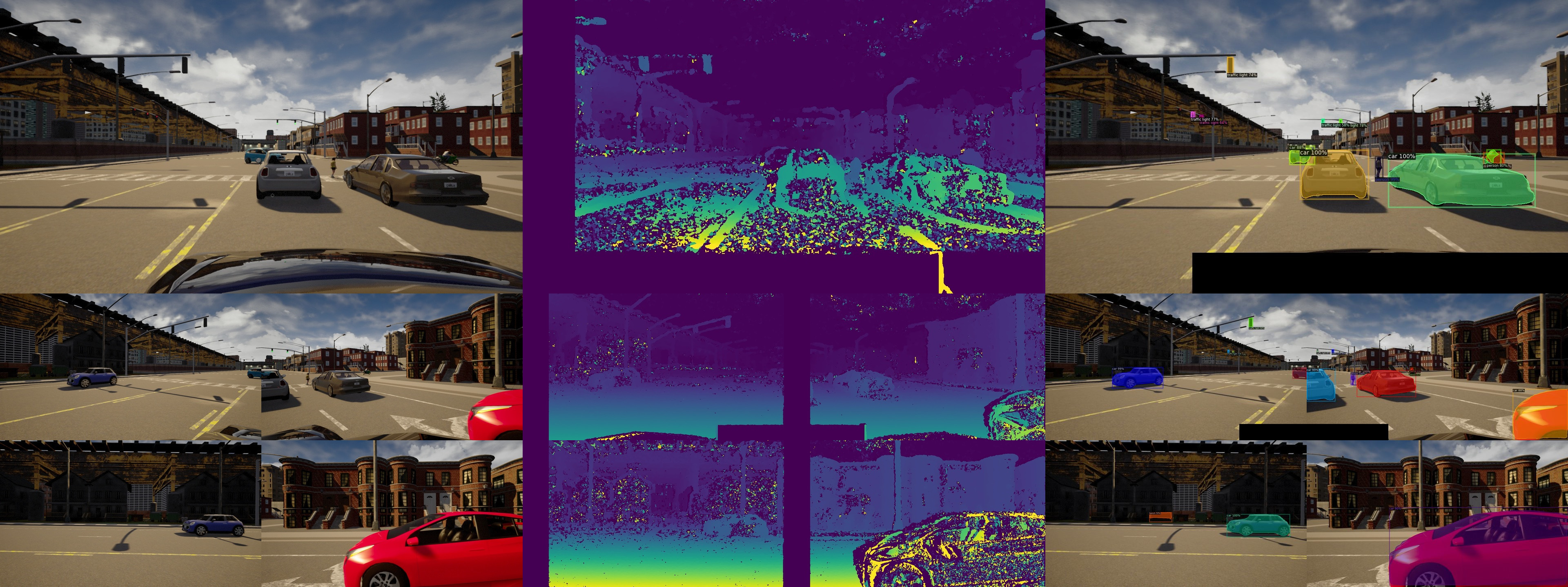
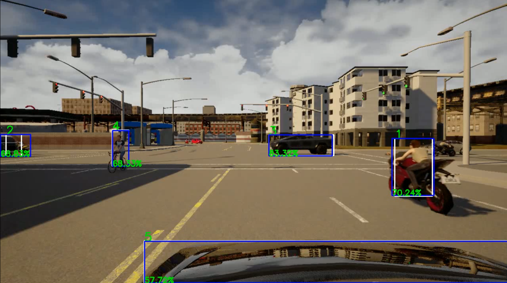
A visualization of the detection results can be seen on
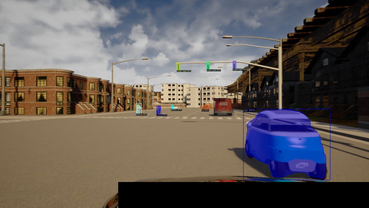
A visualization of the Detectron2 detections and instance segmentation on an ego-occluded image
To perform depth estimation I found to easiest way is to use OpenCV a widely used library in computer vision that includes the stereo processing tools I needed.
OpenCV is a library of programming functions mainly aimed at real-time computer vision originally developed by Intel. The library is cross-platform and free for use. It provides traditional Computer Vision tools such as the stereo correspondence algorithm using block matching (Hamzah, Hamid, and Salim 2010) and an advanced version of it the Semi-Global Block Matching method (SGBM) (Hirschmuller 2008) that I used for the stereo disparity map calculation.
The Stereo Block Matching Algorithm works by comparing the neighborhood of a pixel to each neighborhood of the row of the other image - the measure of similarity can be different, but usually the mean squared error is used. Usually before using the stereo block matchin algorithm a camera calibration is required. This happens with the chessboard calibration method11 where a flat checkerboard is displayed in front of the two stereo cameras. The calibration algorithm then calculates the distortion for each camera and rotation difference between the two cameras to calculate the intrinsic matrix.
In our case since we record images in a super ideal way: no distortion and perfectly parallel cameras we don’t need any calibration and application of inverse intrinsic matrix before using the SGBM algorithm.
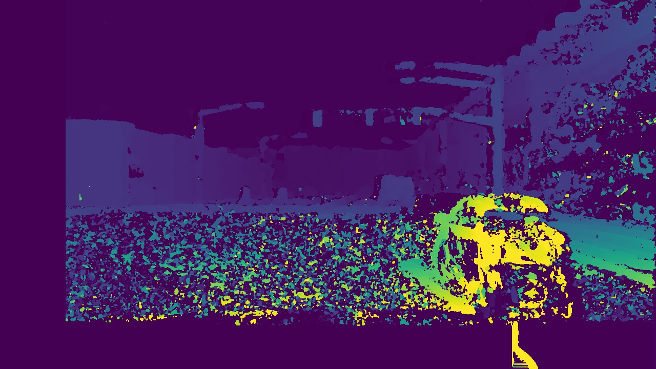
A visualized disparity map result after using OpenCV’s StereoSGBM algorithm on the front stereo side
The StereoBM algorithm considers the left image as the primary, so it will return a disparitymap that corresponds to the pixels of the left image.
Triangulation is a simple method of deriving the depth coordinate when we have two parallel cameras. shows the camera setting of an ideal stereo setting. Recall, that each stereo side in our setting is like this.
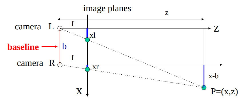
An ideal parallel stereo camera model.
If there is a point P in the real world in the field of view of the stereo camerase, the point will be projected onto different points of both camera’s image plane. If the cameras are set in an ideal parallel stereoscopic setting then we can easily calculate the depth of the point. The pixel difference between between pixels correspoonding to the same block can be calculated with xr-xl. The OpenCV Stereo BM algorithm provides this value for each matched pixel. From now on all we have to do is use triangulation to calculate the depth of each pixel. The f corresponds to the focus length and Z corresponds to the real depth of the point.
The following equations hold true for the figure above from similar triangles. \[\begin{aligned} \begin{split} \frac{z}{f} = \frac{x}{xl} = \frac{x-b}{xr} \\ \frac{z}{f} = \frac{y}{yl} = \frac{y-b}{yr} \end{split}\end{aligned}\]
From this the triangulation is as follows:
\[\begin{aligned} \begin{split} \text{Depth}\;\; Z = \frac{f \cdot b}{xl - xr} = \frac{f \cdot b}{disparity} \\ X = \frac{xl \cdot z}{f} \\ Y = \frac{yl \cdot z}{f} \end{split} \label{eq:depthcalc}\end{aligned}\]
Where xl and yl refers to to distance from the center of the image to the center points of the detection boundingbox (in the left image).
Now we know the way to calculate the depth knowing the disparity. The result of the SGBM, seen on , is a 2D array containg valid and invalid data values. In order to determine the right disparity value for a detection it is not enough to simple take the values under the mask. The disparities under a mask contain values for the same object’s closest point and farthest point from the camera. Taking into account the simplifications we established in the previous chapter there are two solutions to find the distance of the object: 1.) take the average of the valid disparities under a mask 2.) take the mode of the disparities. By intuition we would choose taking the average, however that is going to result in high error and high variance. The reason is, that the segmentation itself is going to mask values that might not correspond to the object’s disparities. Even a few values that are far from the average the object’s disparities can change the average of the masked disparities drastically. Using the mode the algorithm yielded much more stable results, that way it simply is ignores the small inaccuracies of the masking and disparity error and takes the most dominant disparity value. The visualization of masking can be seen on .
Masking the instance segmentation with the disparitymap filters the necessary values for estimating the vehcile’s depth
Each stereo side has a transformation matrix initialized before running the algorithm. Each matrix is an affine 4x4 transformation matrix, that does the following in this order:
It swapes the axes from the image coordinate system to Carla’s coordinate system z->x, x->y, y->z
It rotates the points with the same rotation as the camera
It translates the camera with the same translation for the camerase relative to the vehcile’s bottom center point.
The resulting x, y, z coordinates are the final detection coordinates that go into the detection log.
The final algorithm pseudo-code:
for each frame:
            for each stereo side:
                1. read left and right image
                2. occlude ego from image
                3. compute disparity map using stereo bm.
                4. predict detections and instance segmentation
                for each detection:
                    mask disparity map with detection segmentation
                    calculate mode of the masked disparity
                    apply triangulation and inverse projection
                    add actor to frame
            add frame to framelist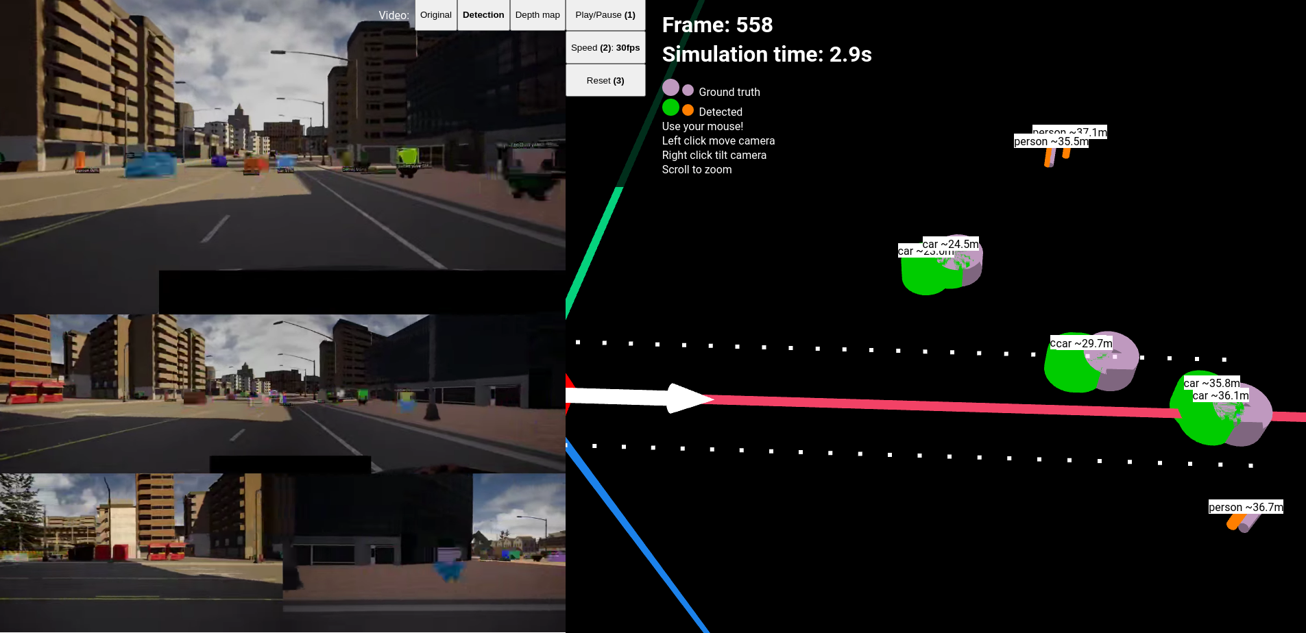
save detection listAs I mentioned before in order to compare the detection result and the ground truth log of each rendering scenario it would be useful to have a visusalization of the detection replayed. This is similar to the information shown on a monitor of a self-driving car.
Since I already had experience in Javascript and in ReactJs12 - an easy-to-use web application framework developed by Facebook - I decided to look for options in 3D visualization. I found WebViz13, a React library specifically made for 3D visualization of traffic scenarios. It has a compelling declarative API.
There are two main views in the end product webvisualizer: The video montage and the 3D visualization
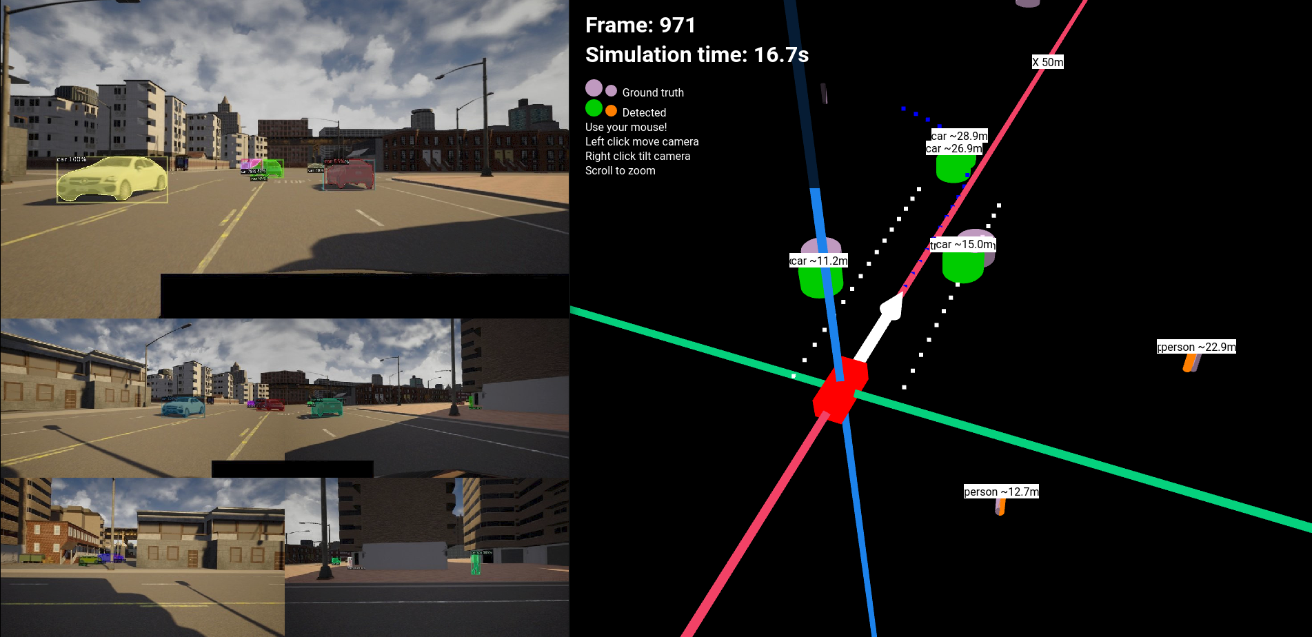
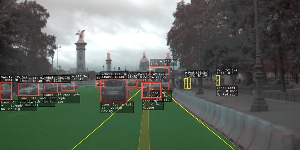
The main feature of the webvisualizer is to replay each simulation and see the original, detection and depthmap videos in synchronization with the 3D visualizer that displays both the detection log and the ground truth log for each frame. The webapp is equipped with control buttons that help the control of the playback.
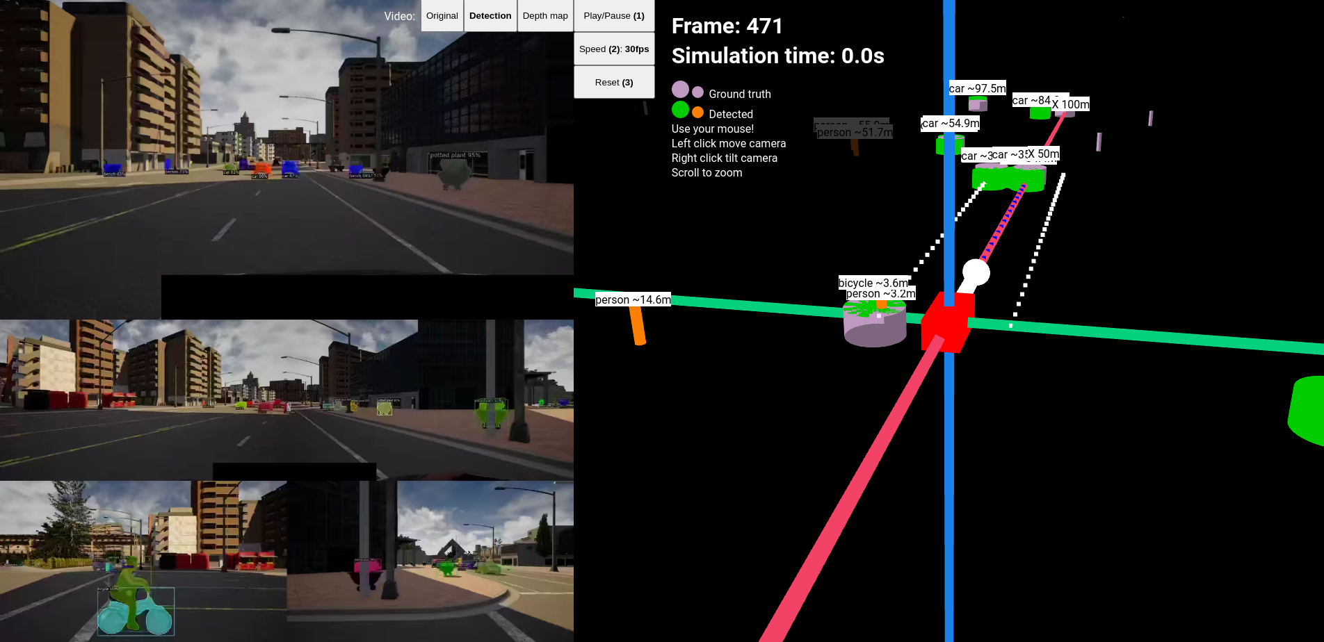
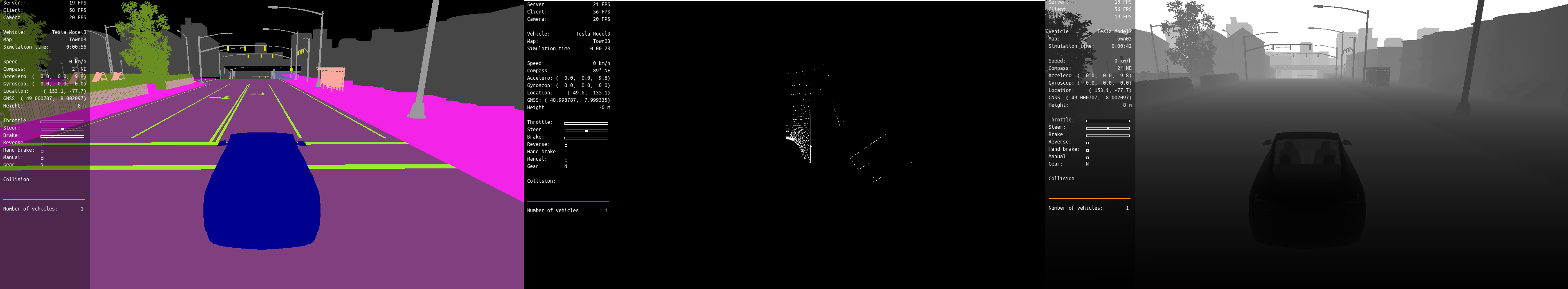
Screenshot of the webvisualizer
The montage videos in the webvisalization: original, depthmap, detections
In order to simplify some tasks that included multiple repetitive commands I had to create some scripts that let me invoke them in one command. One script was to start the simulator, the ego controller and spawn actors in a choosen map all in one script. Another useful script was to create a montage of all frames and immediately create a video and compress it multiple times.
The best way to see the accuracy of the detector is through the webvisualizer. The reader is encouraged to visit https://najibghadri.com/msc-thesis/ where you can interact with with the simulation playback and see each detection.
The reader might notice that most of the time the detected objects are located closer than the ground truth. Recall, that the depth estimation happens on the surface of the object. Estimating the centerpoint is difficult. If instead of working with centerpoints I would have worked with a more complex approach of first detection orientation or 3D bounding box, ther would be no need for working with center points. I discuss improvements later on.
General accuraccy of the detector visualized in the webviewer
Genearlly there are no missed objects but there are false positives. Most of the detections are accurate within 0.5meters.
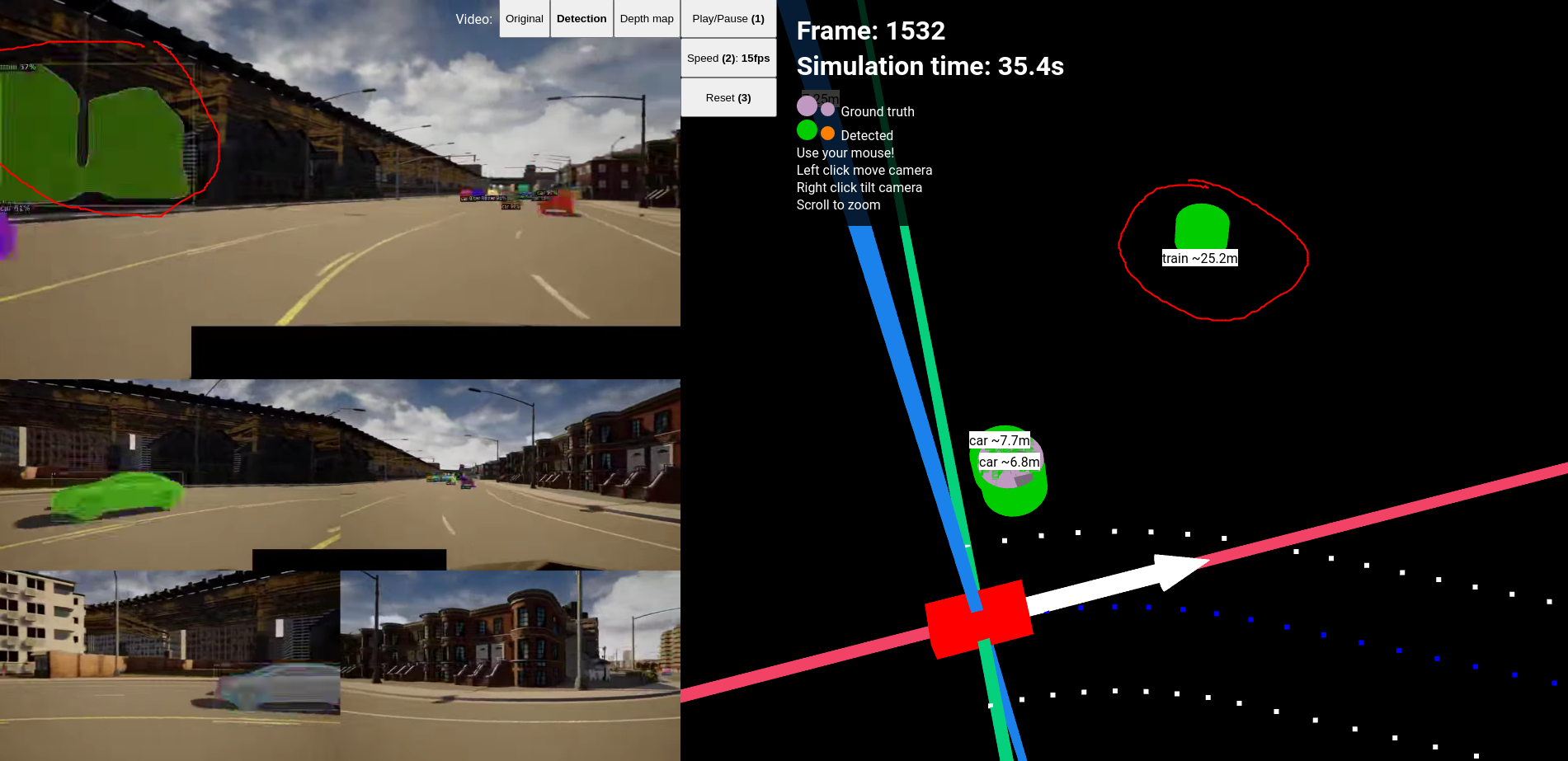
False positive detection where a building is detected as a train
Depth estimation is not accurate enough due to the inaccuracy of the blockmatching algorithm. This can be fixed with the use of LiDAR or radio sensors instead of stereo imaging. Optimal sensor suite is discussed in Improvements .
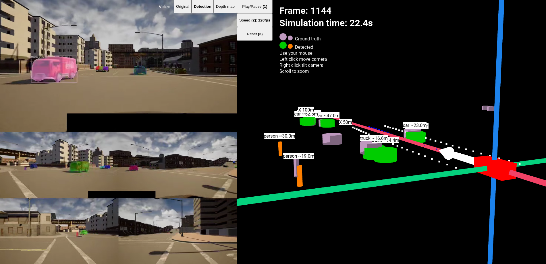
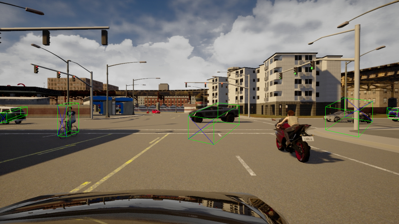
Since the setero sides overlap and they see different sides of the detect objects in the detection log the objects appear as many times as many sides it appears on as seen on . This can be fixed by using tracking and using a shared feature dictionary. Another solution is to abandon stereo camera based depth estimation and use mono cameras with radio or LiDAR sensors for depth estimation with cameras having a small overlapping region. This would be similar to Tesla’s approach.
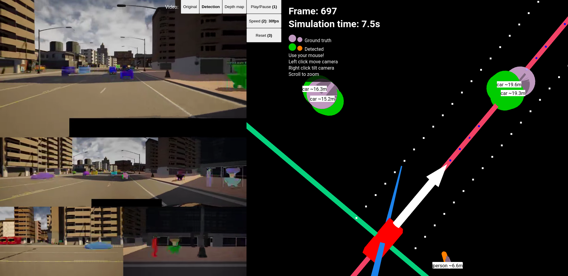
Multiple detections of the same object due to overlapping stereo sides
Despite these depth estimation can be accurate to 70 meters even as seen on .
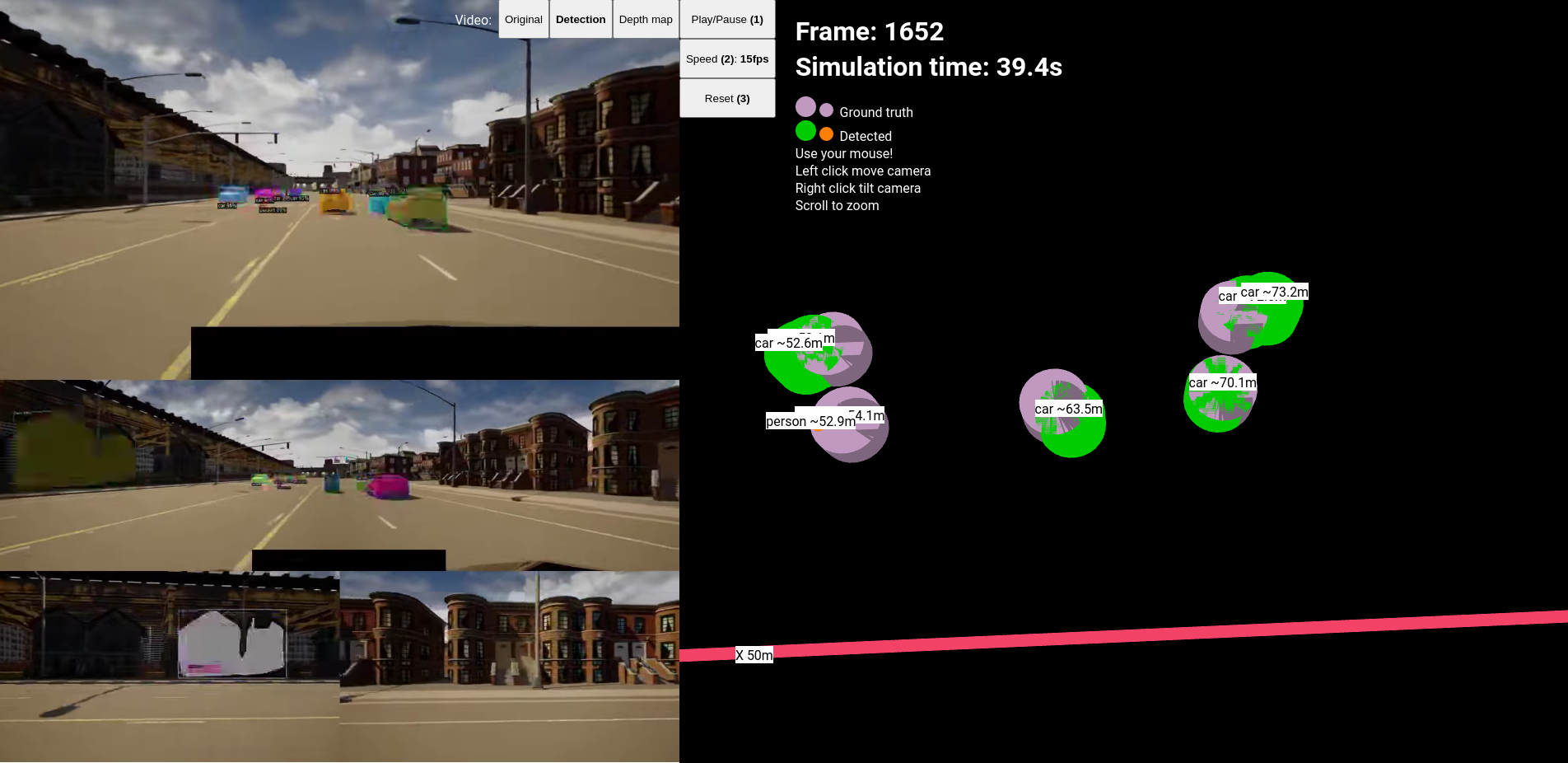
Relatively accurate depth estimation for far distances of ~70 meters
An automatic quantification method for the error will be discussed in .
Choosing different convnet models for Detectron2 can change the performance and accuracy of the detector. I used the ResNet-101 model (He et al. 2015). ResNet50 is faster but I experienced more detection misses.
| Sides | FPS average | |
|---|---|---|
| All 5 sides | 0.53 FPS | |
| One side | 2.73 FPS |
[tab:TabularExample]
In imporvements on instance segmentation research will be discussed that might lead to an improved detection speed over Detectron2.
As discussed earlier in about assumptions, the Z coordinate (in Carla UE coordinates ) is disgregarded in the webvisualization. The accuracy of the Z coordinate is not worse or better the X and Y coordinates but it doesn’t add information and due to an inconsistency in CARLA simulator when returning the location of actors for vehicles and pedestriands the center point is interpreted differently. Hence it showed a false inaccuracy in the Z direction, however not significant as seen on .
Inaccuracies on the Z coordinates are not significant
In on imporvements a different more complex and robust approach to position estimation is discussed that doesn’t use detected bounding box centerpoints.
There is only one map with a “night” situation, and it takes place in a city that is well-luminated, hence I don’t consider it a night light test, but it is darker than other scenarios. The results are good no significant objects were missed.
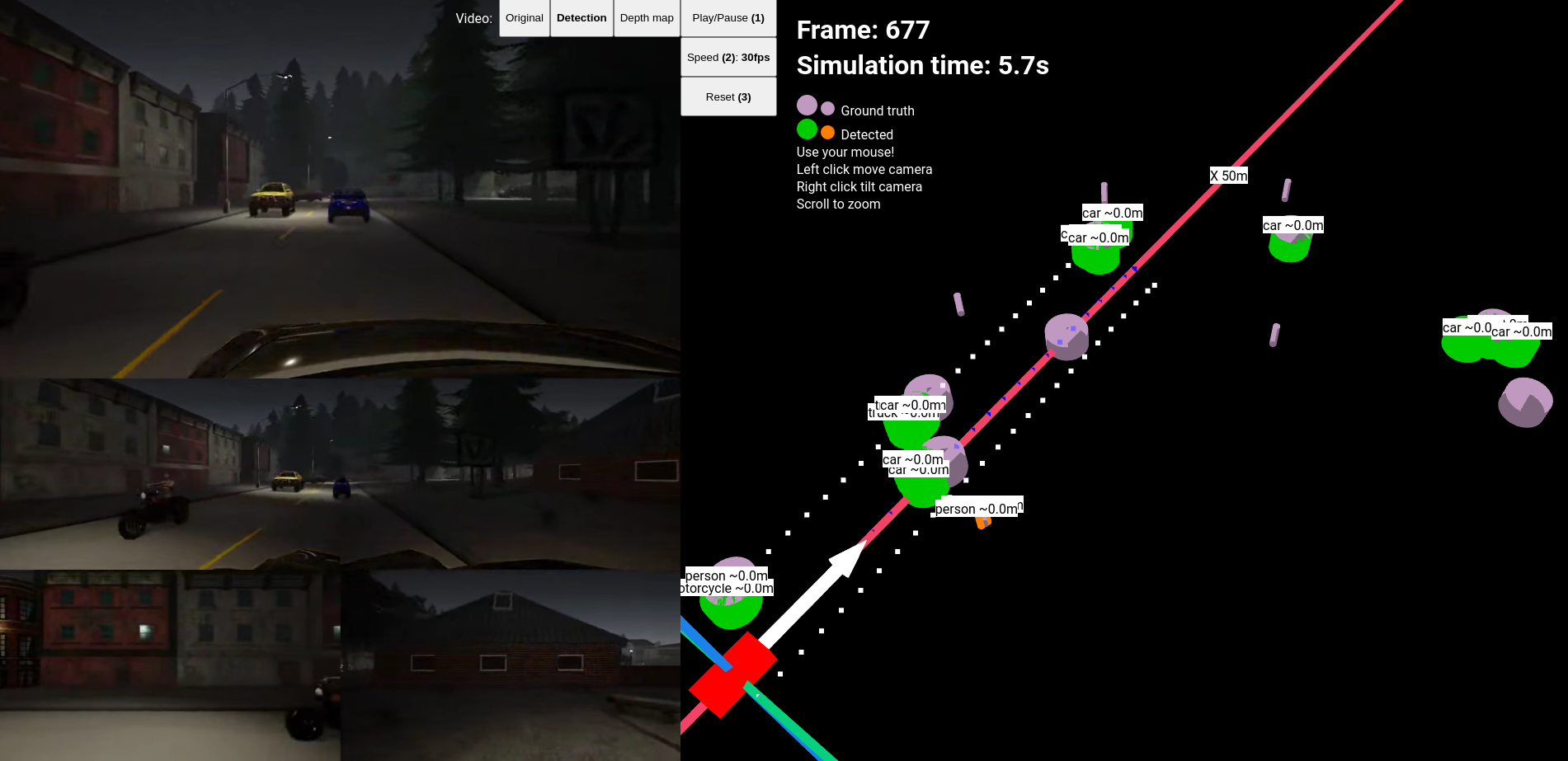
Night situation yields good performance
It wasn’t possible for me to evalute the real-timeness of the system simply because the architecture doesn’t allow that. As discussed earlier in Nvidia Drive Consteallation has support for HIL simulation that could be used to test the real-timeness of systems.
In I established some simplifications to the system. In order to create a fully capable scene understanding algorithm the following improvements are necessary.
In order to measure the accuracy of detections (false positives, false negatives), it is important to correlate the positive detections with the most likely ground truth actor. This could be done by finding the closest truth actor to each detection. There is no point in implementing more robust solutions, because if the error is so high that there are conflicting possibilities for the nearest possible truth object then the depth estimation is fundamentally flawed.
A new research has emerged relating instance segmentation, YOLACT (Bolya et al. 2019a) and YOLACT++ (Bolya et al. 2019b)14, that achieves 30+fps on Titan X for instance segmentation and detection. It is based on YOLO and uses the same resnet50 model that Detectron2 uses. If this convnet achieves the same accuracy with a higher fps than it is replaceable with Detectron2.
We have seen that companies use many sensors combined not only rgb cameras. In an optimal setting I would use only one stereo camera setting to the front and rely on radar and ultrasonic sensors for depth data. Monodepth (Godard, Mac Aodha, and Brostow 2017) is also an option to estimate or correct depth however it might not be a stable method.
Keypoint or landmark based orientation estimation would be a robust method to determine the orientation of vehicle in an image. This is imporant in order to determine which side is visible to the depth map, and assign the depth data to that side of the object and reconstruct knowing this information. In the next chapter I describe to methods I experimented with to estimate orientation.
The percieved information must be corrected with the car’s gyroscopic data, because cameras get tilted. This is important when the road we are on or the road ahed of us has a high difference in inclination.
Lane detection can be done with the prevalent methods such a Hough transform combined with sliding window curve fit. Another possibility is to take into account the vehicles in front and behind us and interpret their path as the right path and regress the lane to their path. However this might lead to uninteded results.
With the usage of sonar and radar sensors and even more so with LiDAR it is possible to detect object on the road. However it is more robust if the algorithm can detect when there is an object on the road independent of what it is exactly. A solution to this would be to use road segmentation which has to exclude segmenting the foreign object on the road creating a hole in the segmentation.
Traffic light understanding is a straightforward problem to have. Detection algorithm trained on the COCO (Lin et al. 2014) dataset are already able to detect traffic lights. A difficult problem to solve is if there are multiple traffic lights visible to the camera, but even then, usually the closest one facing towards the vehicle is the one to follow. After determining the traffic light we have to read the current value, which is a simple image processing procedure. Optionally if this is not enough the algorithm can be made more robust by teaching a convnet to be able to determine the position of the three light circles.
Detecting traffic officers could also be a useful part of the algorithm. There are new human pose estimation algorithms that could even help in understanding the gestures of an officer controlling the road.
One of the most exciting improvement after all improvements above have been achieved is to research and implement Energy based models for self-driving cars, I recommend reading the paper “A tutorial on energy-based learning” (Lecun et al. 1998) by Yann LeCun et al.
Initially I wanted to use YOLOv4 (Bochkovskiy, Wang, and Liao 2020) as the sole detection algorithm. YOLO is indeed realtime however it only provides 2D bounding boxes of the detections which is not enough when we need to mask the depth map with an instance segmentation.
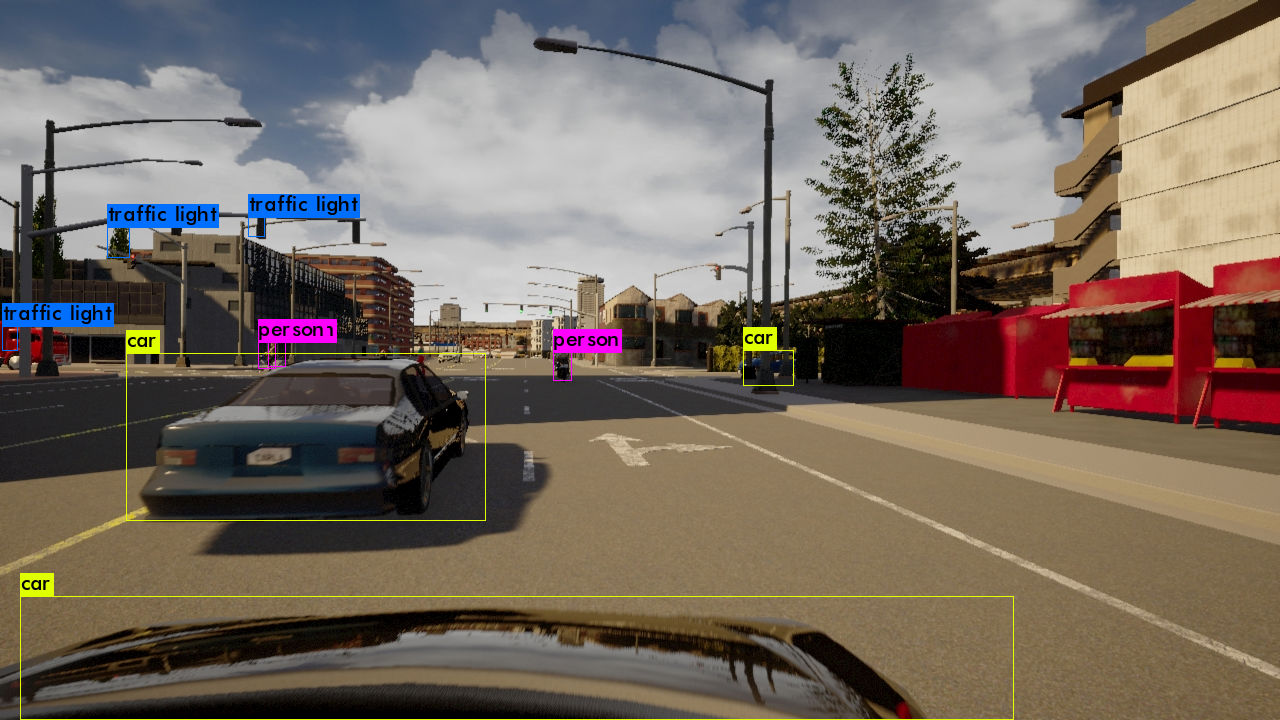
YOLOv4 under evaluation
As mentioned previously it is essential to track objects throught time. I tested Deep SORT (Wojke and Bewley 2018) algorithm which is an improvement over Simple Online and Realtime Tracking (SORT) (Wojke, Bewley, and Paulus 2017). This building block ended upnot being in the detector however a following version will certainly need a tracker method.
Deep SORT also works with Kalman filters and it needs detection instances to predict identites over time. Each bounding box is provided to the tracker which then creates a signature of the detection based on it’s pixel values and then calculates distances with other previously dtected object from a dictionary. A single counter is incremented for each new object that couldn’t be correlated with the previously detected objects.
I evaluated test using YOLOv4 as the detector. Results of a test video can be seen in
Screenshot during a video being processed by the tracker.
When I experimented with lane detection I once tried to use a neural network for the task. Hough transform and sliding window technique could have been enough but I was curious of the accuracy on the simulator.
“Towards End-to-End Lane Detection: an Instance Segmentation Approach” (Caesar et al. 2019) is a neural network that basically works as an edge detector that is directed towards the vanishing point in the image. Note the if the network had been trained it might have yielded better results! In the results of the original paper the results were better but the training data was specific to a certain road.
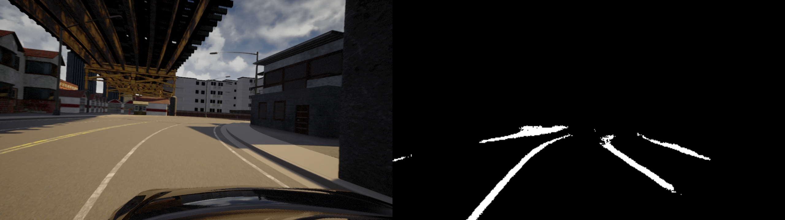
Lane detection performed well without training
As mentioned earlier as an essential imporvement over the current algorithm. I evaluated two approaches. The first approach is direct 3D bounding box detection the second is keypoint detection.
Direct orientation estimation would be an important part of the detector as mentioned previously in improvements. Before implementing the detector I tried a CNN implementation15 based on the paper “3D Bounding Box Estimation Using Deep Learning and Geometry” (Mousavian et al. 2016). This network works similarly to landmark detection but it adds geometric constraints to regress the orientation of the bounding boxes.
Bounding box detection performed poorly. Note, that YOLOv3 missed the motorcycle, thus it is not predicted
After the previous approach failed next idea was that we could derive the orientation of the vehicles if we knew the position of it’s keypoints/landmarks in the images. After some research I found a research developed at Google AI “Discovery of Latent 3D Keypoints via End-to-end Geometric Reasoning” or KeypointNet (Suwajanakorn et al. 2018).
The netowrk performed poorly on CARLA vehicles. I tried with and without instance segmentation but the results seemed independent.
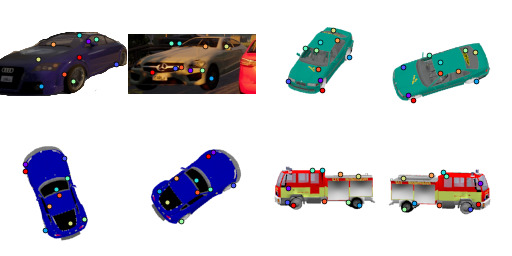
Keypoint detection on CARLA vehicles was inaccurate
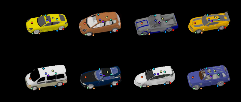
Expected results (from https://keypointnet.github.io/)
The final scene understanding algorithm is not a system that can be applied by itself in a real scenario, however it builds on the same basic ideas for scene understanding for cars. More importantly this thesis helped me understand the building blocks required for autonomous driving. The work of companies like Tesla and Waymo constitues many top researchers in the field. In Hungary this market is in early stages yet, but companies like BOSCH or a smaller company like AIMotive are already present and working on the field with a good pace.
Working on this thesis has been a unique experience because the whole field was new to me before diving into it. Usually thesis projects require that the student works on the same project for 4 semesters, however I had to take a different path. I did my previous research work in Web Applications and applied blockchain technology. Then I took an optional a deep learning class and it sparked my interest for AI even more. Taking this project was a risk and I had to learn about basic computer vision processing methods, algorithms, 3D vision, the camera model, convolutional neural networks and deep learning and even a little bit of game engines because of the simulator. But in the end I learned valueable things and I hope I can use this knowledge soon in an AI company perhaps one that works on autopilots.
Most importantly I want to thank my family for the all-time support. I would also like to thank my closest friends. I would like to thank my supervisor, PhD student, Márton Szemenyei for the help, trust, and the counseling I got during creating this project. I would also like to thank my previous supervisor Dr. Balázs Goldschmidt for his support in work I had done before starting this project.
Bochkovskiy, Alexey, Chien-Yao Wang, and Hong-Yuan Mark Liao. 2020. “YOLOv4: Optimal Speed and Accuracy of Object Detection.” ArXiv abs/2004.10934.
Bolya, Daniel, Chong Zhou, Fanyi Xiao, and Yong Jae Lee. 2019a. “YOLACT: Real-time Instance Segmentation.” In ICCV.
2019b. “YOLACT++: Better Real-Time Instance Segmentation.”
Caesar, Holger, Varun Bankiti, Alex H. Lang, Sourabh Vora, Venice Erin Liong, Qiang Xu, Anush Krishnan, Yu Pan, Giancarlo Baldan, and Oscar Beijbom. 2019. “NuScenes: A Multimodal Dataset for Autonomous Driving.” CoRR abs/1903.11027. http://arxiv.org/abs/1903.11027.
Cordts, Marius, Mohamed Omran, Sebastian Ramos, Timo Rehfeld, Markus Enzweiler, Rodrigo Benenson, Uwe Franke, Stefan Roth, and Bernt Schiele. 2016. “The Cityscapes Dataset for Semantic Urban Scene Understanding.” In Proc. of the Ieee Conference on Computer Vision and Pattern Recognition (Cvpr).
Dosovitskiy, Alexey, German Ros, Felipe Codevilla, Antonio Lopez, and Vladlen Koltun. 2017. “CARLA: An Open Urban Driving Simulator.” In Proceedings of the 1st Annual Conference on Robot Learning, 1–16.
Girshick, Ross B. 2015. “Fast R-CNN.” CoRR abs/1504.08083. http://arxiv.org/abs/1504.08083.
Girshick, Ross B., Jeff Donahue, Trevor Darrell, and Jitendra Malik. 2013. “Rich Feature Hierarchies for Accurate Object Detection and Semantic Segmentation.” CoRR abs/1311.2524. http://arxiv.org/abs/1311.2524.
Godard, Clément, Oisin Mac Aodha, and Gabriel J. Brostow. 2017. “Unsupervised Monocular Depth Estimation with Left-Right Consistency.” In CVPR.
Hamzah, R. A., A. M. A. Hamid, and S. I. M. Salim. 2010. “The Solution of Stereo Correspondence Problem Using Block Matching Algorithm in Stereo Vision Mobile Robot.” In 2010 Second International Conference on Computer Research and Development, 733–37.
He, Kaiming, Georgia Gkioxari, Piotr Dollár, and Ross B. Girshick. 2017. “Mask R-CNN.” CoRR abs/1703.06870. http://arxiv.org/abs/1703.06870.
He, Kaiming, Xiangyu Zhang, Shaoqing Ren, and Jian Sun. 2015. “Deep Residual Learning for Image Recognition.” CoRR abs/1512.03385. http://arxiv.org/abs/1512.03385.
Hirschmuller, H. 2008. “Stereo Processing by Semiglobal Matching and Mutual Information.” IEEE Transactions on Pattern Analysis and Machine Intelligence 30 (2): 328–41.
“J3016B: Taxonomy and Definitions for Terms Related to Driving Automation Systems for on-Road Motor Vehicles - SAE International.” 2020. Accessed May 28. https://www.sae.org/standards/content/j3016_201806/.
Krizhevsky, Alex, Ilya Sutskever, and Geoffrey E Hinton. 2012. “ImageNet Classification with Deep Convolutional Neural Networks.” In Advances in Neural Information Processing Systems 25, edited by F. Pereira, C. J. C. Burges, L. Bottou, and K. Q. Weinberger, 1097–1105. Curran Associates, Inc. http://papers.nips.cc/paper/4824-imagenet-classification-with-deep-convolutional-neural-networks.pdf.
Lecun, Yann, Léon Bottou, Yoshua Bengio, and Patrick Haffner. 1998. “Gradient-Based Learning Applied to Document Recognition.” In Proceedings of the Ieee, 2278–2324.
Lin, Tsung-Yi, Michael Maire, Serge J. Belongie, Lubomir D. Bourdev, Ross B. Girshick, James Hays, Pietro Perona, Deva Ramanan, Piotr Dollár, and C. Lawrence Zitnick. 2014. “Microsoft COCO: Common Objects in Context.” CoRR abs/1405.0312. http://arxiv.org/abs/1405.0312.
Liu, Wei, Dragomir Anguelov, Dumitru Erhan, Christian Szegedy, Scott E. Reed, Cheng-Yang Fu, and Alexander C. Berg. 2015. “SSD: Single Shot Multibox Detector.” CoRR abs/1512.02325. http://arxiv.org/abs/1512.02325.
Long, Jonathan, Evan Shelhamer, and Trevor Darrell. 2014. “Fully Convolutional Networks for Semantic Segmentation.” CoRR abs/1411.4038. http://arxiv.org/abs/1411.4038.
Mousavian, Arsalan, Dragomir Anguelov, John Flynn, and Jana Kosecka. 2016. “3D Bounding Box Estimation Using Deep Learning and Geometry.” CoRR abs/1612.00496. http://arxiv.org/abs/1612.00496.
Simonyan, Karen, and Andrew Zisserman. 2014. “Very Deep Convolutional Networks for Large-Scale Image Recognition.” CoRR abs/1409.1556. http://arxiv.org/abs/1409.1556.
Sun, Pei, Henrik Kretzschmar, Xerxes Dotiwalla, Aurelien Chouard, Vijaysai Patnaik, Paul Tsui, James Guo, et al. 2019. “Scalability in Perception for Autonomous Driving: Waymo Open Dataset.”
Suwajanakorn, Supasorn, Noah Snavely, Jonathan Tompson, and Mohammad Norouzi. 2018. “Discovery of Latent 3d Keypoints via End-to-End Geometric Reasoning.” arXiv:1807.03146 [Cs, Stat], November. http://arxiv.org/abs/1807.03146.
Szegedy, Christian, Wei Liu, Yangqing Jia, Pierre Sermanet, Scott E. Reed, Dragomir Anguelov, Dumitru Erhan, Vincent Vanhoucke, and Andrew Rabinovich. 2014. “Going Deeper with Convolutions.” CoRR abs/1409.4842. http://arxiv.org/abs/1409.4842.
Wojke, Nicolai, and Alex Bewley. 2018. “Deep Cosine Metric Learning for Person Re-Identification.” In 2018 Ieee Winter Conference on Applications of Computer Vision (Wacv), 748–56. IEEE. doi:10.1109/WACV.2018.00087.
Wojke, Nicolai, Alex Bewley, and Dietrich Paulus. 2017. “Simple Online and Realtime Tracking with a Deep Association Metric.” In 2017 Ieee International Conference on Image Processing (Icip), 3645–9. IEEE. doi:10.1109/ICIP.2017.8296962.
Wu, Yuxin, Alexander Kirillov, Francisco Massa, Wan-Yen Lo, and Ross Girshick. 2019. “Detectron2.” https://github.com/facebookresearch/detectron2.
Luminar https://www.luminartech.com/↩
Stanford CV course CS231N https://cs231n.github.io/↩
Tesla Autonomy Day https://www.youtube.com/watch?v=Ucp0TTmvqOE↩
Robot Operating System (ROS) https://www.ros.org/↩
Unreal Engine https://www.unrealengine.com/↩
CARLA sensors reference https://carla.readthedocs.io/en/latest/ref_sensors/↩
Deepdrive Voyage https://deepdrive.voyage.auto/↩
NVIDIA Drive Constellation https://developer.nvidia.com/drive/drive-constellation↩
RFPro http://www.rfpro.com/↩
Titan X GPU https://www.nvidia.com/en-us/geforce/products/10series/titan-x-pascal/↩
Chessboard calibration in OpenCV https://docs.opencv.org/master/dc/dbb/tutorial_py_calibration.html↩
ReactJs https://reactjs.org/↩
WorldView WebViz https://webviz.io/worldview/↩
Yolact++ repository https://github.com/dbolya/yolact↩
3D Bounding Box implementation https://github.com/skhadem/3D-BoundingBox↩